Skin Lesion Analysis Using Convolutional Neural Networks with Transfer Learning
For this class project, the objective was to solve a real-world problem that we were free to choose in teams. Me and my team decided to solve the Skin Lesion Analysis problem, which is an online competetion that is held every year by ISIC. The goal of this project was to develop an intelligent image analysis tool to enable the automated diagnosis of 7 different skin cancer types from dermoscopic images, that is basically a multi-class classification task. Main challenges of the ISIC 2018 dataset that it was multi-class, quite imbalanced and had relatively insufficient samples to train deep neural networks. We have tackled this problem by applying data augmentation techniques and transfer learning. We trained our networks on the original dataset besides the augmented one and consolidated the contributions of our approach.
What I have done briefly:
My responsibility in the team was to handle the drawbacks of the dataset, which were imbalanced characteristics and insufficient amount of data. I came up with several solutions against these such as data augmentation and to transfer learning to train a deep convolutional neural network properly. Instead of implementing a brand new CNN classifier, I used one of the well known networks at the time, called VGG-16, to make some more time for data handling besides learning about the network's architecture. Applying transfer learning basically refers to train a network that has already been trained on another dataset. This is done by keeping some of the learned weights of network fixed while training the rest of its parameters on the target dataset. Therefore, I trained only the fully connected layers along with the last four convolutional layer while retaining the weights of the network's previous layers learned from ImageNet dataset. By keeping the first layers' weights, I utilized the feature extraction abilities of a network which was trained on a huge dataset consisted of over 14 billion images. Training the last group of layers enabled classifier to specialize more on the target dataset and helped me to reduce the effect of having insufficient data for training a deep network. Exploiting transfer learning also lowered the training time as I had to train way fewer parameters.
For the data augmentation part, I spent much more time to visually analyze random images from the dataset in order to decide which augmentation techniques would be suitable. After a time-taking research on determining what were the beneficial techniques for my case, I have implemented and applied those as described in the data preprocessing section. I explained my approach step-by-step under the data augmentation title in the same section.
Both techniques I've described helped us to prevent our models from both overfitting and low class-based classification accuracies which were very important for such a cancer classification task.
Details on Dataset
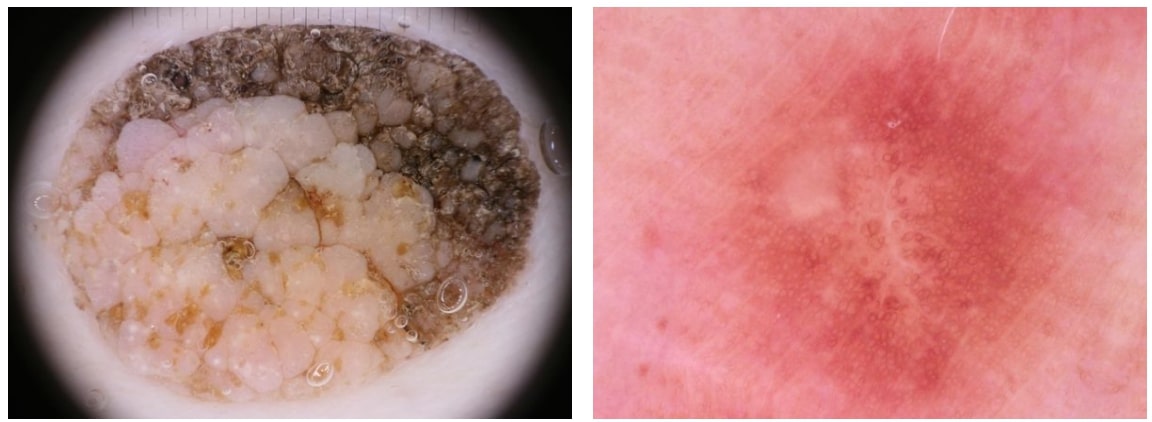
Our data was extracted from the ISIC 2018 (ISIC 2018: Skin Lesion Analysis Towards Melanoma Detection) grand challenge datasets. Training data for the last challenge consisted of 10015 RGB lesion images that had the size of 450x600 and associated file with labels for seven disease categories which are Melanoma (MEL), Melanocytic nevus (NV), Basal cell carcinoma (BCC), Actinic keratosis / Bowens disease- intraepithelial carcinoma (AKIEC), Benign keratosis- solar lentigo / seborrheic keratosis / lichen planus-like keratosis (BKN), Dermatofibroma (DF) and Vascular lesion (VASC). Additionally, we were given supplemental information about images in the dataset that included image identifier with associated lesion identifier and diagnosis confirm type. Images with the same lesion identifier showed the alike primary lesion on a patient, as mentioned on the challenge forum. There are a couple of drawbacks of this dataset as it is highly imbalanced and contains a considerable number of noisy images. Number of instances for each class is shown in Table 1 to reveal their disproportion. The noise on the other hand can be described as the reflections of measurement units or the scope borders on the images which caused inconsistent lesion imaging. A pair of noisy and normal image is demonstrated in Figure 1, in which noisy image has a measure scale on top and scope borders in corners. Moreover, since challenge committee did not provide the labels for validation and test sets during the competetion time, I had to split training set into train, validation and test sets. Since classification scores are originally tested on 1157 images in the competetion, I chose the same instance numbers as our validation and test set numbers.
| MEL | NV | BCC | AKIEC | BKN | DF | VASC |
|---|---|---|---|---|---|---|
| 1113 | 6704 | 514 | 327 | 1099 | 115 | 142 |
Data Preprocessing
Image Augmentation
I can summarize my approach toward image augmentation as below.
- I first counted the number of pictures belonging to each class before starting any model development in order to see if I had a balanced or imbalanced dataset
- Then realized the dataset was highly imbalanced as already mentioned, therefore I decided to perform image augmentation
- To determine how many extra samples I had to generate by augmentation, I took the class with least instances into consideration and determined the required number of augmented images per real image existed in that class. In other words, I've equalized the number of samples in each class by augmenting images respectively
- Visually analyzed random images from the dataset in order to decide on appropriate augmentation techniques
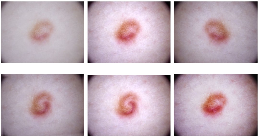
- Read the skimage.transformation library documentation and decided to use rotation, flip up-down and left-right, noise, contrast, brightness, and sigmoid correction which I believed perfectly suited to this specific dataset of skin lesion images
- Experimented with each of these techniques and figured out the proper parameter intervals for each of these image processes. For example, our rotation angle is chosen from a +45 -45 degrees interval and swirling strength is from 0 to 3 in magnitude.
- Wrote a script which produced brand new images from the original ones, randomly selecting processing parameters from the intervals I have defined in the previous step. These pictures are produced by 15 combinations of the above explained augmentation methods
- Applied this to all minority classes, and down-sampled the majority class into a reasonable level
- Separated all classes into respective folders and splitted them as train-validation-test sets
Finally, I ended up with an augmented dataset of 3k instances for each class, forming up an enhanced and balanced new dataset containing approximately 21k images. The positive outcome of my data augmentation approach was confirmed by the validation accuracy graphs of same network, trained separately both on augmented and the original dataset to determine the effect of image augmenting.
Data Augmentation Code
import pandas as pd
import numpy as np
from skimage import io
from skimage.util import random_noise
from skimage.transform import rotate, resize, swirl
from skimage import exposure
import matplotlib.pyplot as plt
from tqdm import tqdm
def plt_im(image):
    plt.imshow(image)
    plt.show()


def image_to_np(row, dataframe, plot=False):
    im_name = dataframe['image'][row]
    image = io.imread("./data/ISIC2018_Training_Input/" + im_name + ".jpg")

    if plot:
        plt.imshow(image)
        plt.show()

    return np.array(image)


def brighten(image):
    return exposure.adjust_gamma(image, gamma=0.5, gain=0.9)


def sigmoid(image):
    return exposure.adjust_sigmoid(image, gain=7)


def swirl_im(image, strength=3):
    return swirl(image, mode='reflect', radius=300, strength=strength)


def contrast(image):
    v_min, v_max = np.percentile(image, (0.4, 99.6))
    better_contrast = exposure.rescale_intensity(image, in_range=(v_min, v_max))
    return better_contrast


def random_rotation(image):
    # pick a random degree of rotation between 45 deg on the left and 45 deg on the right
    random_degree = np.random.uniform(-25, 25)
    return rotate(image, random_degree, mode='symmetric')


def augment_data(class_id, image_indexes, dataframe):
    """
    :param class_id: Integer in [0-6] representing a specific class.
    :param image_indexes: List storing image names for each class.
    :param dataframe: Dataframe storing GroundTruth table (image names and labels).
     Finally save the augmented dataset.
    """
    print('cls ID: ', class_id)
    idx = image_indexes[class_id]
    if class_id == 2:
        strt = 360
    if class_id == 4:
        strt = 959

    print('strt: ', strt)

    for i in tqdm(range(strt, len(idx)), desc="Data augmentation"):

        im = image_to_np(idx[i], dataframe)
        plt.imsave('./augmented/cls{}/cls{}_{}_ud.jpg'.format(class_id, class_id, i), np.flipud(im))
        plt.imsave('./augmented/cls{}/cls{}_{}_lr.jpg'.format(class_id, class_id, i), np.fliplr(im))
        plt.imsave('./augmented/cls{}/cls{}_{}_rotate.jpg'.format(class_id, class_id, i), random_rotation(im))
        plt.imsave('./augmented/cls{}/cls{}_{}_noise.jpg'.format(class_id, class_id, i), random_noise(im))
        plt.imsave('./augmented/cls{}/cls{}_{}_contrast.jpg'.format(class_id, class_id, i), contrast(im))
        plt.imsave('./augmented/cls{}/cls{}_{}_bright.jpg'.format(class_id, class_id, i), brighten(im))
        plt.imsave('./augmented/cls{}/cls{}_{}_swirl.jpg'.format(class_id, class_id, i), swirl_im(im))
        plt.imsave('./augmented/cls{}/cls{}_{}_sigmoid.jpg'.format(class_id, class_id, i), sigmoid(im))

        plt.imsave('./augmented/cls{}/cls{}_{}_swirl_rot.jpg'.format(class_id, class_id, i), random_rotation(swirl_im(im, strength=2)))
        plt.imsave('./augmented/cls{}/cls{}_{}_swirl_rot_bri.jpg'.format(class_id, class_id, i), brighten(random_rotation(swirl_im(im, strength=2.5))))
        plt.imsave('./augmented/cls{}/cls{}_{}_swirl_rot_contr.jpg'.format(class_id, class_id, i), contrast(random_rotation(swirl_im(im, strength=3))))
        plt.imsave('./augmented/cls{}/cls{}_{}_swirl_sig.jpg'.format(class_id, class_id, i), sigmoid(swirl_im(im, strength=2)))
        plt.imsave('./augmented/cls{}/cls{}_{}_rot_lr.jpg'.format(class_id, class_id, i), random_rotation(np.fliplr(im)))
        plt.imsave('./augmented/cls{}/cls{}_{}_rot_ud.jpg'.format(class_id, class_id, i), random_rotation(np.flipud(im)))
        plt.imsave('./augmented/cls{}/cls{}_{}_rot_contr.jpg'.format(class_id, class_id, i), random_rotation(contrast(im)))


def separate_images_into_class_folders():
    """
    Separate images of each class and save to Balanced_Trainset folder.

    """
    for i in range(len(im_idx)):
        print('class in operation: ', i)
        for j in tqdm(range(len(im_idx[i]))):
            #if i != 1:
            img = image_to_np(im_idx[i][j], df)
            plt.imsave('./data/Balanced_Trainset/cls{}/{}.jpg'.format(i, df['image'][im_idx[i][j]]), img)
df = pd.read_csv('./data/ISIC2018_Training_GroundTruth.csv')
labels = np.array(df.iloc[:, 1:]).astype(int)

# image_names = []
im_idx = []
for i in range(labels.shape[1]):
    print('Class {} instances: {}'.format(i+1, np.count_nonzero(np.where(labels[:, i] == 1))))
    indexes = np.argwhere(labels[:, i] == 1)
    indexes = indexes.squeeze()
    im_idx.append(indexes)
    # image_names.append(df['image'][indexes].tolist())


# Augmentation
augment_data(5, im_idx, df)
augment_data(6, im_idx, df)
augment_data(3, im_idx, df)
augment_data(2, im_idx, df)
augment_data(0, im_idx, df)
augment_data(4, im_idx, df)
Classifier
Mainly I did:
- Implement the convolutional neural network VGG16 as the feature extractor
- Test with pretrained weights on the original dataset and achieved only around 50% accuracy
- Flatten the output of the network and add a fully connected layer in order to have it more specialized on the target dataset
- Train last four convolutional layers along with this added fully connected layer, performing a grid search with number of nodes [64, 128, 512, 1024] and dropout factor of [0.3, 0.4, 0.5]. Also experiment with the learning rate [0.01, 0.001, 0.0001], momentum [0.9], and decay [1e-5, 1e-6] parameters
- Realize adding random zoom in and out operation increased the accuracy, so implement built-in zoom factor during training
- Achieve more than 90% of classification accuracy with the parameters reported
- Experiment with the same parameter setups both on imbalanced and balanced (augmented) dataset
- Report the class-based precision, recall, f1-score metrics on both balanced and imbalanced datasets to confirm the improvement in minority classes. See results section.
Classifier Code
I used Keras to use the pre-trained convolutional network.
from keras.applications import VGG16
from keras import models
from keras import layers
from keras import optimizers
from keras import metrics
from keras.preprocessing.image import ImageDataGenerator
import matplotlib.pyplot as plt
import os
import pandas as pd
Setup the Input and Output Directories
train_dir = "./data/balanced_trainset"
validation_dir = "./data/Validation_set"
test_dir = "./data/Validation_set/"
model_save_name = "lastt_50epoch_relu_vgg16_imnet_Dense64"
acc_figure_title = "_VGG16 Accuracy - Imnet Transfer Learning"
loss_figure_title = "_VGG16 Loss - Imnet Transfer Learning"
do_save = False
num_epoch = 50
Load the VGG16 Network
Get the pre-trained network and freeze the layers except last four.
vgg_conv = VGG16(weights='imagenet', include_top=False, input_shape=(224, 224, 3))

# Freeze the layers except the last 4 layers
for layer in vgg_conv.layers[:-4]:
    layer.trainable = False

# Check the trainable status of the individual layers
for layer in vgg_conv.layers:
    print(layer, layer.trainable)


#%% Construct the whole model
# Create the model
model = models.Sequential()

# Add the vgg convolutional base model
model.add(vgg_conv)

# Add new layers
model.add(layers.Flatten())
model.add(layers.Dense(128, activation='relu'))
model.add(layers.Dropout(0.3))
model.add(layers.Dense(7, activation='softmax'))

# Make model parallel.
#model = multi_gpu_model(model, gpus=7)

# Show a summary of the model. Check the number of trainable parameters
model.summary()
Setup the Data Generator
Since number of images are high enough to not to fit in memory, we should use data generators to read image data on the fly.
train_batchsize = 18
val_batchsize = 8

train_datagen = ImageDataGenerator(rescale=1. / 255,
                                   rotation_range=20,
                                   zoom_range=0.2,
                                   width_shift_range=0.2,
                                   height_shift_range=0.2,
                                   fill_mode='nearest')

validation_datagen = ImageDataGenerator(rescale=1./255)
'''                                     rotation_range=20,
                                        zoom_range=0.2,
                                        width_shift_range=0.2,
                                        height_shift_range=0.2,
                                        horizontal_flip=True,
                                        fill_mode='nearest')
'''

train_generator = train_datagen.flow_from_directory(
    train_dir,
    target_size=(224, 224),
    batch_size=train_batchsize,
    class_mode='categorical')

validation_generator = validation_datagen.flow_from_directory(
    validation_dir,
    target_size=(224, 224),
    batch_size=val_batchsize,
    class_mode='categorical',
    shuffle=False)
print('\nData Generators are ready---------')
Train the Model
sgd = optimizers.SGD(lr=0.001, decay=1e-6, momentum=0.9, nesterov=True)

# Compile the model
model.compile(loss='categorical_crossentropy',
              optimizer=sgd,
              metrics=['acc'])


# Train the model
history = model.fit_generator(
    train_generator,
    steps_per_epoch=train_generator.samples / train_generator.batch_size,
    epochs=num_epoch,
    validation_data=validation_generator,
    validation_steps=validation_generator.samples / validation_generator.batch_size,
    verbose=1)

print('\nTraining completed---------')
# Save the model
if do_save:
    model.save("./models/" + model_save_name + ".h5")
Evaluate the Model
print('\nEvaluation Started------------------')

test_datagen = ImageDataGenerator(rescale=1./255)

test_generator = test_datagen.flow_from_directory(
    directory=test_dir,
    target_size=(224, 224),
    color_mode="rgb",
    batch_size=1,
    class_mode='categorical',
    shuffle=False,
    seed=42
)
print('Test generator created. Prediction is starting..')

test_generator.reset()
pred = model.predict_generator(test_generator,verbose=1)

print('Saving prediction results..')
pd.DataFrame(pred, columns=['MEL', 'NV', 'BCC', 'AKIEC', 'BKL', 'DF', 'VASC']).to_csv('vgg16_pred.csv')

print('Saved.')

# Save Plots
acc = history.history['acc']
val_acc = history.history['val_acc']
loss = history.history['loss']
val_loss = history.history['val_loss']

epochs = range(len(acc))

plt.plot(epochs, acc, 'b', label='Training acc')
plt.plot(epochs, val_acc, 'r', label='Validation acc')
plt.title('VGG16 Training and Validation Accuracy')
plt.xlabel('Epochs')
plt.ylabel('Accuracy')
plt.legend()

plt.savefig("./out_graphs/" + acc_figure_title +  ".png", bbox_inches='tight')


plt.figure()

plt.plot(epochs, loss, 'b', label='Training loss')
plt.plot(epochs, val_loss, 'r', label='Validation loss')
plt.title('VGG16 Training and Validation Loss')
plt.xlabel('Epochs')
plt.ylabel('Loss')
plt.legend()

plt.savefig("./out_graphs/" + loss_figure_title +  ".png", bbox_inches='tight')

#plt.show()
print('Plots are saved.')

print('Process finished.')
Results
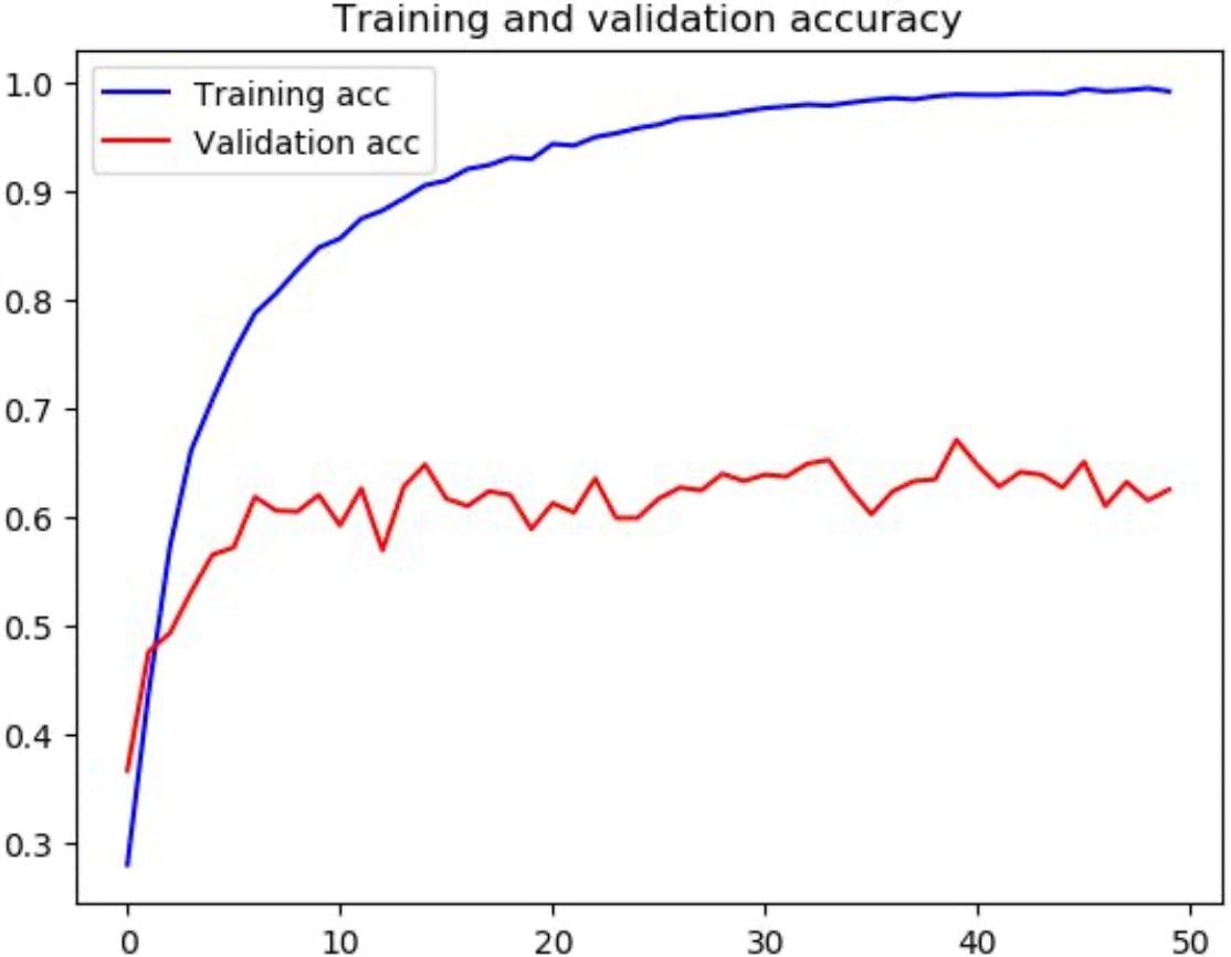
The positive outcome of my approaches was confirmed by the train-validation accuracy graphs of same network, trained separately both on augmented and the original dataset to determine the effect of image augmenting.
Here in figure 3, we can clearly say that the network is overfitted to the train set, reaching almost a perfect classification result on it while barely making it around 60% of accuracy on the validation set.
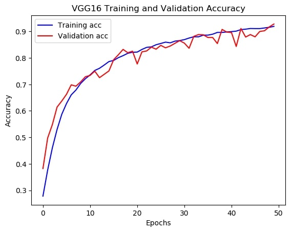
By contrast, the same network performed much better on validation set with a classification score of about 92% after being trained on the augmented train set. Demonstrated in figure 4.
Since the classification of minority classes was the main idea behind augmenting the data, we lastly need to check on how class-based metrics went. We can get a quite useful report for concerning this analysis by simply employing sklearn.metrics.classification_report().
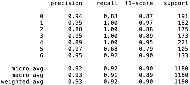
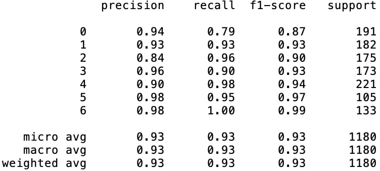
Analyzing the two classification reports in figures 5 and 6, the results draw us the picture of high leaps in class-based accuracies of the minority classes. Besides improving all of the minority classes' $(\text{class}_2, \text{class}_3, \text{class}_5, \text{class}_6)$ f1-scores, especially the increase in $\text{class}_5$ score seems like a remarkable development which is increased from 79% to 97%.