Gaussian Mixture Models as Bayesian Classifier

We studied different covariance models for mixtures of Gaussians. Implement the Expectation-Maximization algorithm for these mixtures with the following models:

1. Different spherical covariance matrix for each component
2. Different diagonal covariance matrix for each component
3. Different arbitrary covariance matrix for each component

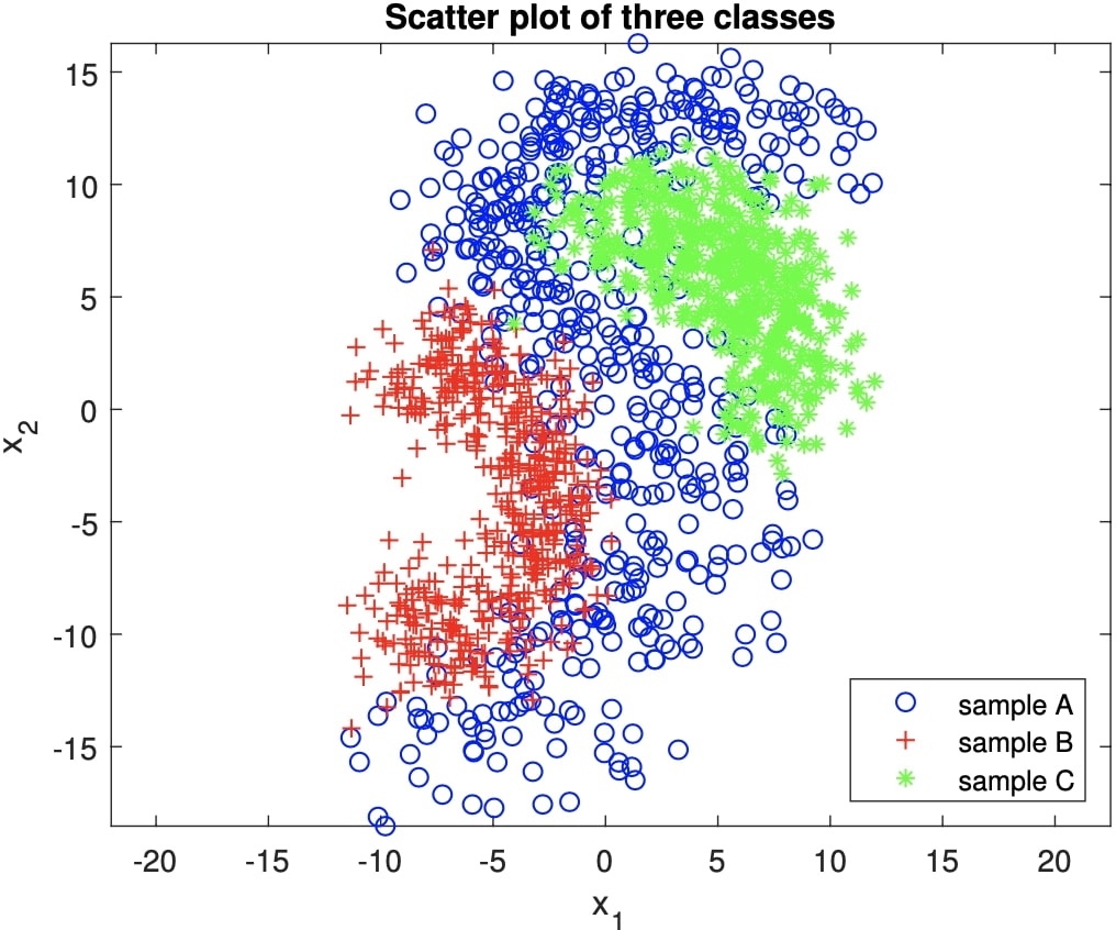
Then, train a Bayesian classifier where each class-conditional probability density is estimated using a mixture of Gaussians for the dataset shown in Figure 1.

Figure 1. Dataset consists of three classes of 1000 observations each. Each observation has two features.

My Approach:

I randomly sampled 500 data points from all of the classes and save them in corresponding txt files for consistency. My policy for fitting the mixture model was like the following:

1. Plot and observe data for choosing an optimal starting point for the gaussian means.
   • For this step, I decided on putting my initial mean points somewhere close to the points I desired to end up around. That way, I reduced the number of iterations for waiting them to fit exact good points.
2. Analyze dataset and determine how many gaussian models would best represent each class individually.
   • I explored data by plotting, and decided on number of gaussian models that would represent them most accurately. For this purpose, my criteria was to observe the curved regions where data tends to twist as the critical points. Hence, I decided to fit gaussians on the each side of those curves.
3. For the stopping condition of the EM algorithm, I experimented with different threshold values and concluded to choose 0.001 as the threshold representing the latest log-likelihood difference.

Histogram-Based Bayesian Classifier

Implement a Bayesian classifier where the class-conditional probabilities are estimated using histograms.

My Approach:

1. Create three 2d-histogram tables with respect to the three individual classes using my hist() method. All three histogram tables have to be identical in dimension and starting-ending points. Therefore use minimum and maximum values of overall training data, and use the same bin number taken from the user.
2. Determine number of data from each class that involves in every cell.
3. Obtain probabilities of each class holds for every cell in the grid.
4. Stack all three histograms in z-dimension and compare (argmax) each identical cell on axis 2 (z-dimension)
5. Assign labels according to these probabilities, choosing the dominant one for each cell. At the end of this step, bayesian_decision_grid is formed.
6. Take data to be predicted, fit onto the bayesian_decision_grid, assign corresponding labels to data. Finally, histogram_predicted list created, which stores the predicted labels.
7. Evaluate prediction results comparing to the true labels, print accuracies and confusion matrices for training and the test sets.

Implementation

import numpy as np
from numpy.linalg import inv, det
import matplotlib.pyplot as plt
from scipy.stats import multivariate_normal
from sklearn.metrics import confusion_matrix,accuracy_score

Helper Functions

def decision_grid(hist_tables):
    # Stack all three 2d-histograms to determine bayesian decision on each cell.
    hist_tables = np.dstack((hist_tables[0], hist_tables[1], hist_tables[2]))
    # Create bayesian decision grid (labels).
    decision_table = hist_tables.argmax(axis=2)
    return decision_table


def hist_predict(X, bayesian_decision_grid, bin_num):

    predicted = np.zeros(len(X))

    min_x1, min_x2 = np.min(X, axis=0)
    max_x1, max_x2 = np.max(X, axis=0)

    x1_range = np.abs(max_x1 - min_x1)
    x2_range = np.abs(max_x2 - min_x2)

    x1_divided = np.array([np.arange(min_x1, (max_x1 + x1_range / bin_num), x1_range / bin_num)]).T
    x2_divided = np.array([np.arange(min_x2, (max_x2 + x2_range / bin_num), x2_range / bin_num)]).T

    indexes = []
    for i in range(bin_num):
        for j in range(bin_num):
            indexes.append(np.nonzero((x1_divided[i] < X[:, 0]) & (X[:, 0] < x1_divided[i + 1]) & (x2_divided[j] < X[:, 1]) & (X[:, 1] < x2_divided[j + 1]))[0])
            if indexes[-1].size != 0:
                predicted[indexes[-1]] = bayesian_decision_grid[i][j] + 1  # Add one to avoid zero index.
    return predicted.astype(int)


def prob(X, gauss):
    prob_list = np.empty((X.shape[0], 1))
    Xmu = (X - gauss.mu)  # X - mu

    for i in range(X.shape[0]):
        density = gauss.alpha * (1 / ((2 * np.pi) * np.sqrt(det(gauss.sigma)))) + \
                  (-0.5 * np.dot(Xmu[i, :].dot(inv(gauss.sigma)), Xmu[i, :].T))
        prob_list[i] = density
    return prob_list


def predict(X, mixture_models):
    gauss_models = []
    class1_labels = np.arange(len(mixture_models[0].gausses))
    class2_labels = np.arange(class1_labels[-1] + 1, len(mixture_models[1].gausses) + class1_labels.shape[0])
    class3_labels = np.arange(class2_labels[-1] + 1,
                              len(mixture_models[2].gausses) + class1_labels.shape[0] + class2_labels.shape[0])

    for i in range(len(mixture_models)):
        for j in range(len(mixture_models[i].gausses)):
            gauss_models.append(mixture_models[i].gausses[j])

    bayes_table = np.empty((X.shape[0], len(gauss_models)))
    for i, g in zip(range(len(gauss_models)), gauss_models):
        bayes_list = prob(X, g)
        bayes_table[:, i] = bayes_list.ravel()

    bayes_table = np.exp(bayes_table)
    bayes_table = bayes_table / np.sum(bayes_table, axis=1)[:, np.newaxis]
    decision = bayes_table.argmax(axis=1)

    for i in range(len(X)):
        if np.isin(decision[i], class1_labels):
            decision[i] = 1
        elif np.isin(decision[i], class2_labels):
            decision[i] = 2
        elif np.isin(decision[i], class3_labels):
            decision[i] = 3
        else:
            print('No decision!!')
    return decision


def evaluate(true_labels, predicted, cm=False):
    acc = accuracy_score(true_labels, predicted)
    if cm == False: return acc
    else:
        cm = confusion_matrix(true_labels, predicted)
        return acc, cm


def plot_gauss_locs(gauss_list, new_figure=False):
    """
        Plot the mean coordinates of given gaussian distribution(s).
        gauss_list: list of gauss objects.
    """
    if new_figure:
        plt.figure()

    x1_loc = []
    x2_loc = []
    for g in gauss_list:
        x1_loc.append(g.mu[0])
        x2_loc.append(g.mu[1])

    plt.scatter(x1_loc, x2_loc, c='black')
    plt.axis('equal')
    plt.show()
    print('\nGauss locations plotted. Amount: ', len(gauss_list))


def plot_covariance(gauss, all=False):

    x_line = np.linspace(-20, 20, 1000)
    y_line = np.linspace(-20, 20, 1000)
    xx, yy = np.meshgrid(x_line, y_line)
    pos = np.empty(xx.shape + (2,))
    pos[:, :, 0] = xx
    pos[:, :, 1] = yy
    if not all:
        rv = multivariate_normal([gauss.mu[0], gauss.mu[1]], [gauss.sigma[0], gauss.sigma[1]])
        plt.contour(xx, yy, rv.pdf(pos), colors='k', alpha=0.3)
    else:
        for gmm in gauss:
            for g in gmm.gausses:
                rv = multivariate_normal([g.mu[0], g.mu[1]], [g.sigma[0], g.sigma[1]])
                plt.contour(xx, yy, rv.pdf(pos), colors='k', alpha=0.3)

    plt.axis('equal')
    plt.show()


def plot_data(data, row=-5, new_figure=False, all=True):
    """
        Plot given data easily.
        data: 2D data array.
        If row specified, prints that row only.
    """
    color = ['bs', 'go', 'r^']
    if new_figure:
        plt.figure()
    if not all:
        if row == -5:
            plt.plot(data[:, 0], data[:, 1], color[0], markersize='1')
        else:
            plt.plot(data[row, 0], data[row, 1], 'r^', markersize='1')
    else:
        for d in range(len(data)):
            plt.plot(data[d][:, 0], data[d][:, 1], color[d], markersize='1')
    plt.axis('equal')
    plt.show()
    print('\nData plotted.')


def plot_loglikelihood(GMM):
    plt.figure()
    plt.plot(GMM.loglikelihood_record[1:])
    plt.xlabel('Number of iterations')
    plt.ylabel('Loglikelihood values')

Gaussian Mixture Model

This class creates a gaussian mixture model given their paramaters $\mu$ and $\beta$ and fits to the training data by means of Expectation-Maximization algorithm.

class GMM:
    def __init__(self, mu_list, sigma_list, covariance_type):

        self.sigma_list = sigma_list
        self.mu_list = mu_list
        self.num_of_models = len(mu_list)
        self.alpha_list = self.init_alpha_list(self.num_of_models)
        self. covariance_type = covariance_type

        self.gausses = self.create_gauss_models(self.mu_list, self.sigma_list, self.alpha_list, self.num_of_models)
        self.prob_table = []
        self.current_loglike = 1
        self.loglikelihood_record = [0]
        self.threshold = 0.00001
        self.d = 0  # dimension is set in fit_mixtures method.

    def create_gauss_models(self, mu_list, sigma_list, alpha_list, num_of_models):
        if len(sigma_list) != num_of_models:
            print('MU_LIST AND SIGMA_LIST HAS TO BE THE SAME SIZE!')

        gausses = []
        for i in range(num_of_models):
            gausses.append(Gauss(mu_list[i], sigma_list[i], alpha_list[i]))
        return gausses


    def init_alpha_list(self, num_of_models):
        a_list = []
        alpha = 1/np.round(num_of_models, decimals=3)
        for i in range(num_of_models):
            a_list.append(alpha)
        return a_list


    def expectation(self, X, gauss):

        prob_list = np.empty((X.shape[0], 1))
        Xmu = (X - gauss.mu)  # X - mu
        #print('ZERO FOUND ', np.where(Xmu == 0)[0])

        for i in range(X.shape[0]):
            density = gauss.alpha * (1 / ((2 * np.pi) * np.sqrt(det(gauss.sigma)))) + \
                     (-0.5 * np.dot(Xmu[i, :].dot(inv(gauss.sigma)), Xmu[i, :].T))
            prob_list[i] = density
        return prob_list

    def maximization(self, X, prob_table, gausses):
        d = X.shape[1]
        labels = prob_table.argmax(axis=1)

        '''
        # Plot data belonging to each Gaussian model.
        for i in range(np.unique(labels).size):
            plt.scatter(X[labels == i][:, 0], X[labels == i][:, 1], alpha=0.5)
        
        # Plot means of each Gaussian model.
        mu_plt = np.array([g.mu for g in gausses])
        plt.scatter(mu_plt[:, 0], mu_plt[:, 1])
        plt.show()
        '''

        # Print how many points belong to each Gaussian model.
        #for l in range(np.unique(labels).size):
        #    print('Labels == {} count : {}'.format(l, (labels == l).sum()))

        # M-Step.
        # Updating sigma will change for 3 different cov matrices.
        #if self.covariance_type == 'diagonal': self.covariance_type = 'arbitrary'
        for j in range(len(gausses)):
            sigma_nominator = 0
            mu_nominator = 0
            a = np.sum(prob_table[labels == j][:, j])  # 'a' is the common value of different equations.
            if self.covariance_type == 'spherical':
                sigma_denominator = d * a
            elif self.covariance_type == 'arbitrary' or self.covariance_type == 'diagonal':
                sigma_denominator = a
            gausses[j].alpha = a / X.shape[0]  # Update ALPHA.
            for i in range(len(X[labels == j])):
                if self.covariance_type == 'spherical':
                    sigma_nominator += prob_table[labels == j][i, j]
                                    * np.sum((X[labels == j][i, :] - gausses[j].mu) ** 2)
                elif self.covariance_type == 'arbitrary':
                    sigma_nominator += prob_table[labels == j][i, j]
                                    * np.dot((X[labels == j][i, :] - gausses[j].mu).reshape(2,1),
                                             (X[labels == j][i, :] - gausses[j].mu).reshape(1,2))
                elif self.covariance_type == 'diagonal':
                    for k in range(d):
                        sigma_nominator += prob_table[labels == j][i, j]
                                        * (X[labels == j][i, k] - gausses[j].mu[k])**2

                mu_nominator += prob_table[labels == j][i, j] * X[labels == j][i, :]

            #print('sigma denom: %s' % sigma_denominator)
            if self.covariance_type == 'spherical' or self.covariance_type == 'diagonal':
                gausses[j].sigma = np.identity(len(gausses[j].sigma))
                * (sigma_nominator / sigma_denominator)  # Update SIGMA
            elif self.covariance_type == 'arbitrary':
                gausses[j].sigma = (sigma_nominator / sigma_denominator)
            gausses[j].mu = mu_nominator / a  # Update MU

            gausses[j].mu_record.append(gausses[j].mu)  # Record MU values to track the movement of gauss function.
            gausses[j].sigma_record.append(gausses[j].sigma)

        # Calculate and record log likelihood.
        new_loglike = 0
        for i in range(len(X)):
            temp = 0
            for j in range(len(gausses)):
                temp += gausses[j].alpha * prob_table[i, j]
            new_loglike += np.log(temp)
        self.loglikelihood_record.append(new_loglike)


    def fit_mixtures(self, X):
        prb_table = np.empty((X.shape[0], len(self.gausses)))
        self.d = X.shape[1]
        # Store alpha values.
        #alphas = []
        #for j in range(len(gausses)):
        #    alphas.append(gausses[j].alpha)

        iterations = 0
        while self.threshold < np.abs(self.loglikelihood_record[iterations]-self.current_loglike):
            #print('while: ', np.abs(self.loglikelihood_record[iterations]-self.current_loglike))
            #print(iterations)
            # E - part
            for i, g in zip(range(len(self.gausses)), self.gausses):
                prob_list = self.expectation(X, g)
                prb_table[:, i] = prob_list.ravel()

            prb_table = np.exp(prb_table)
            prb_table = prb_table / (np.sum(self.alpha_list) * np.sum(prb_table, axis=1))[:, np.newaxis]

            # M - part
            self.current_loglike = self.loglikelihood_record[iterations]
            self.maximization(X, prb_table, self.gausses)
            self.prob_table = prb_table

            if iterations > 0:
                print('Loglikelihood: ', self.loglikelihood_record[iterations])

            '''
            if iterations >= 20:
                if self.loglikelihood_record[iterations] < self.loglikelihood_record[iterations-2]:
                    break
            '''
            iterations += 1

        print('\nNumber of iterations: ', iterations)

Individual Gauss Model

This class holds information on every single Gauss Model in the Gaussian Mixture Model.

class Gauss:
    def __init__(self, mu, sigma, alpha):
        self.mu = mu
        self.sigma = sigma
        self.alpha = alpha

        self.initial_params = [mu, sigma, alpha]

        self.sigma_record = []  # For debug purposes. Uncomment under M-step to get the record.
        self.mu_record = []

Histogram-Based Bayesian Classifier

Implement a Bayesian classifier where the class-conditional probabilities are estimated using histograms.

def hist(X, bin_num, min_points, max_points):
    """
        Takes 2d data as X and counts the num of data points falling into the corresponding 2d bins.
        Can be considered as a grid fitted onto the data.
        Columns are features and rows are observations.

        X[0] -> x1 axis
        X[1] -> x2 axis
        bin_num: int
    """
    min_x1, min_x2 = min_points
    max_x1, max_x2 = max_points

    #min_x1, min_x2 = np.min(X, axis=0)
    #max_x1, max_x2 = np.max(X, axis=0)

    x1_range = np.abs(max_x1 - min_x1)
    x2_range = np.abs(max_x2 - min_x2)

    x1_divided = np.array([np.arange(min_x1, (max_x1 + x1_range / bin_num), x1_range / bin_num)]).T
    x2_divided = np.array([np.arange(min_x2, (max_x2 + x2_range / bin_num), x2_range / bin_num)]).T

    count_grid = np.zeros((bin_num, bin_num))
    for i in range(bin_num):
        for j in range(bin_num):
            count_in_cell = np.count_nonzero(
                (x1_divided[i] < X[:, 0]) & (X[:, 0] < x1_divided[i + 1]) &
                (x2_divided[j] < X[:, 1]) & (X[:, 1] < x2_divided[j + 1]))

            count_grid[i][j] += count_in_cell
    return count_grid

Training and Testing the Implemented Models

Fit Gaussian Mixture Model to Class 1

covariance_model = 'arbitrary'  # When needed to set all models.

class1_Traindata = np.loadtxt('./train_test_splits/class1_train.txt')
class1_Xtrain = class1_Traindata[:, :-1]
class1_Ytrain = class1_Traindata[:, -1].astype(int)
print('\nClass1 train data is read.')

mean1 = np.array([0, 0])   # Middle
mean2 = np.array([2.5, 13.5])    # Top
mean3 = np.array([-2, -14])  # Bottom
cov1 = np.array([[10, 0],
                [0, 10]])
cov2 = np.array([[10, 0],
                [0, 10]])
cov3 = np.array([[10, 0],
                [0, 10]])

mean_list = [mean1, mean2, mean3]
cov_list = [cov1, cov2, cov3]

print('Creating GMM for class1..')
GMM_1 = GMM(mean_list, cov_list, covariance_model)

print('Fitting Gaussian mixture to the class1 data..\n')
GMM_1.fit_mixtures(class1_Xtrain)

for i in range(len(GMM_1.gausses)):
    print('\nGauss{} fitted Sigma:\n{}'.format(i+1, GMM_1.gausses[i].sigma))
    print('\nGauss{} fitted Mean:\n{}'.format(i+1, GMM_1.gausses[i].mu))

# Plot loglikelihood.
plot_loglikelihood(GMM_1)
plt.ylabel('GMM_1 Loglikelihood values')
plt.xlabel('Number of iterations')
plt.title('Gaussian mixture1 on class1')

Fit Gaussian Mixture Model to Class 2

class2_Traindata = np.loadtxt('./train_test_splits/class2_train.txt')
class2_Xtrain = class2_Traindata[:, :-1]
class2_Ytrain = class2_Traindata[:, -1].astype(int)
print('\nClass2 train data is read.')

mean1 = np.array([-8, 3])  # upper side
mean2 = np.array([-2.5, -2.5])  # mid side
mean3 = np.array([-9, -12])  # down side

cov1 = np.array([[9, 2],
                [2, 7]])
cov2 = np.array([[9, 2],
                [2, 7]])
cov3 = np.array([[8, 2],
                [2, 6]])

mean_list = [mean1, mean2, mean3]
cov_list = [cov1, cov2, cov3]

print('Creating GMM for class2..')
GMM_2 = GMM(mean_list, cov_list, covariance_model)

print('Fitting Gaussian mixture to the class2 data..\n')
GMM_2.fit_mixtures(class2_Xtrain)

for i in range(len(GMM_2.gausses)):
    print('\nGauss{} fitted Sigma:\n{}'.format(i+1, GMM_2.gausses[i].sigma))
    print('\nGauss{} fitted Mean:\n{}'.format(i+1, GMM_2.gausses[i].mu))

# Plot loglikelihood.
plot_loglikelihood(GMM_2)
plt.ylabel('GMM_2 Loglikelihood values')
plt.xlabel('Number of iterations')
plt.title('Gaussian mixture2 on class2')

Fit Gaussian Mixture Model to Class 3

class3_Traindata = np.loadtxt('./train_test_splits/class3_train.txt')
class3_Xtrain = class3_Traindata[:, :-1]
class3_Ytrain = class3_Traindata[:, -1].astype(int)
print('\nClass3 train data is read.')

mean1 = np.array([9, 1])
mean2 = np.array([1, 9])

cov1 = np.array([[1, 0],
                [0, 1]])
cov2 = np.array([[1, 0],
                [0, 1]])

mean_list = [mean1, mean2]
cov_list = [cov1, cov2]

print('Creating GMM for class3..')
GMM_3 = GMM(mean_list, cov_list, covariance_model)

print('Fitting Gaussian mixture to the class3 data..\n')
GMM_3.fit_mixtures(class3_Xtrain)

for i in range(len(GMM_3.gausses)):
    print('\nGauss{} fitted Sigma:\n{}'.format(i+1, GMM_3.gausses[i].sigma))
    print('\nGauss{} fitted Mean:\n{}'.format(i+1, GMM_3.gausses[i].mu))

# Plot loglikelihood.
plot_loglikelihood(GMM_3)
plt.ylabel('GMM_3 Loglikehood values')
plt.xlabel('Number of iterations')
plt.title('Gaussian mixture3 on class3')

Evaluate Accuracy on Training Data

mixture_models = [GMM_1, GMM_2, GMM_3]

all_Xtrain_data = np.append(class1_Xtrain, class2_Xtrain, axis=0)
all_Xtrain_data = np.append(all_Xtrain_data, class3_Xtrain, axis=0)
all_Ytrain_data = np.append(class1_Ytrain, class2_Ytrain, axis=0)
all_Ytrain_data = np.append(all_Ytrain_data, class3_Ytrain, axis=0)

c1_predicted = predict(class1_Xtrain, mixture_models)
c2_predicted = predict(class2_Xtrain, mixture_models)
c3_predicted = predict(class3_Xtrain, mixture_models)
train_predicted = predict(all_Xtrain_data, mixture_models)

c1_acc = evaluate(class1_Ytrain, c1_predicted)
c2_acc = evaluate(class2_Ytrain, c2_predicted)
c3_acc = evaluate(class3_Ytrain, c3_predicted)
train_acc, train_cm = evaluate(all_Ytrain_data, train_predicted, cm=True)

print('\nFor training data --------------------------------')
print('\nclass1 acc: {} | class2 acc: {} | class3 acc: {}'.format(c1_acc, c2_acc, c3_acc))
print('overall trainset acc: {}\nconfusion matrix:\n{}'.format(np.round(train_acc, 3), train_cm))

Evaluate Accuracy on Test Data

class1_Testdata = np.loadtxt('./train_test_splits/class1_test.txt')
class1_Xtest = class1_Testdata[:, :-1]
class1_Ytest = class1_Testdata[:, -1].astype(int)
class2_Testdata = np.loadtxt('./train_test_splits/class2_test.txt')
class2_Xtest = class2_Testdata[:, :-1]
class2_Ytest = class2_Testdata[:, -1].astype(int)
class3_Testdata = np.loadtxt('./train_test_splits/class3_test.txt')
class3_Xtest = class3_Testdata[:, :-1]
class3_Ytest = class3_Testdata[:, -1].astype(int)


all_Xtest_data = np.append(class1_Xtest, class2_Xtest, axis=0)
all_Xtest_data = np.append(all_Xtest_data, class3_Xtest, axis=0)
all_Ytest_data = np.append(class1_Ytest, class2_Ytest, axis=0)
all_Ytest_data = np.append(all_Ytest_data, class3_Ytest, axis=0)

c1_predicted = predict(class1_Xtest, mixture_models)
c2_predicted = predict(class2_Xtest, mixture_models)
c3_predicted = predict(class3_Xtest, mixture_models)
test_predicted = predict(all_Xtest_data, mixture_models)

c1_acc = evaluate(class1_Ytest, c1_predicted)
c2_acc = evaluate(class2_Ytest, c2_predicted)
c3_acc = evaluate(class3_Ytest, c3_predicted)
test_acc, test_cm = evaluate(all_Ytest_data, test_predicted, cm=True)

print('\nFor test data ------------------------------------')
print('\nclass1 acc: {} | class2 acc: {} | class3 acc: {}'.format(c1_acc, c2_acc, c3_acc))
print('overall testset acc: {}\nconfusion matrix:\n{}'.format(np.round(test_acc, 3), test_cm))

Plot All Data with Fitted Mixture Models on Top of Them

plt.figure()
plot_data([class1_Xtrain, class2_Xtrain, class3_Xtrain])
plot_gauss_locs(GMM_2.gausses)
plot_covariance(GMM_2.gausses[0])
plot_covariance(GMM_2.gausses[1])
plot_covariance(GMM_2.gausses[2])

#plot_data(class3_Xtrain, all=False)
plot_gauss_locs(GMM_3.gausses)
plot_covariance(GMM_3.gausses[0])
plot_covariance(GMM_3.gausses[1])

#plot_data(class1_Xtrain, all=False)
plot_gauss_locs(GMM_1.gausses)
plot_covariance(GMM_1.gausses[0])
plot_covariance(GMM_1.gausses[1])
plot_covariance(GMM_1.gausses[2])
plt.title('Mixtures Fitted on Training Data')
#plot_covariance(GMM_1.gausses[3])

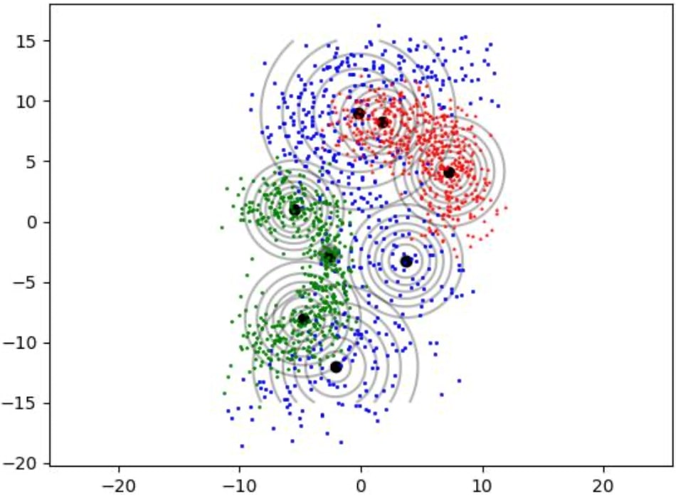
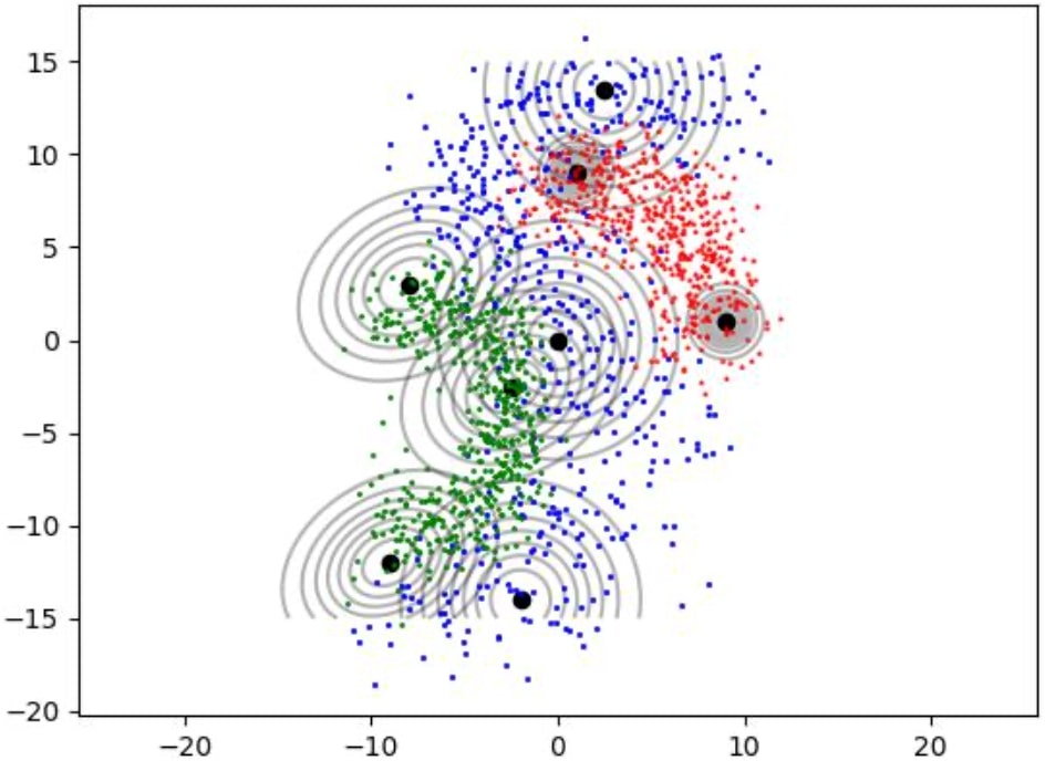
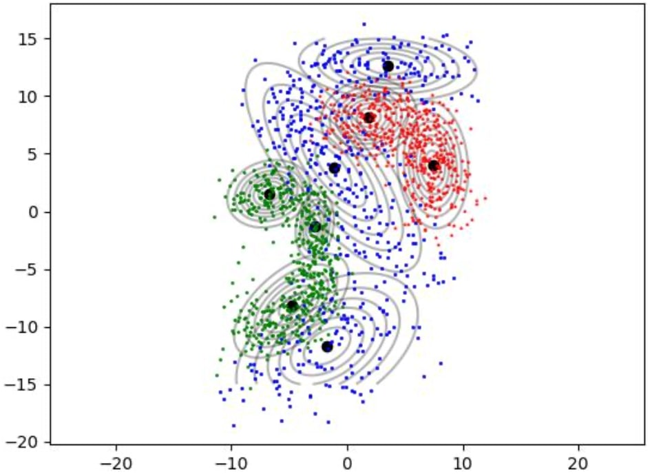
How Gaussian mixture models are fitted to train data as shown in figures 1, 2 and 3.

Figure 2. Some problems with Spherical Gaussian mixtures fitted on all 3 classes. Note that the models fitted on blue and red classes severely interfere with each other, resulting in critical mis-classification of these two classes. Also the green class has a gaussian model that could not fit properly

Figure 3. Arbitrary Gaussian mixtures BEFORE fitted on all the classes

Figure 4. Arbitrary Gaussian mixtures AFTER fitted on all the classes

Discussion on Mixture Models:

During my experiments with different Gaussian mixture models, I observed that arbitrary models were outperforming the other two covariance models. This was quite expected considering the flexible characteristics of the arbitrary covariance matrix, especially differing in the updates at the maximization step. However, one should be careful to choose initial mean and sigma values, as it's easy to end up with undesired fitting results caused by singularity cases or the over-kill. If you choose one mean on the data and the others further away, the EM algorithm will more likely end up with a single gaussian covering all the data points. Therefore, observing data and thinking about the options at the beginning is an essential according to my experiences in this work.

Fit Histogram-Bayesian Classifier

bin_num1 = 40

# Determine a global grid size for all classes.
grid_start, grid_end = np.min(all_Xtrain_data, axis=0), np.max(all_Xtrain_data, axis=0)
# Create 2d-histogram tables for each class.
c1_hist = hist(class1_Xtrain, bin_num1, grid_start, grid_end)
c2_hist = hist(class2_Xtrain, bin_num1, grid_start, grid_end)
c3_hist = hist(class3_Xtrain, bin_num1, grid_start, grid_end)

# Add all tables into a list for decision grid method input.
histogram_tables = [c1_hist, c2_hist, c3_hist]
# Bayesian labels from histograms.
bayesian_decision_grid = decision_grid(histogram_tables)

# Bayesian prediction.
histogram_predicted = hist_predict(all_Xtrain_data, bayesian_decision_grid, bin_num1)
# Evaluate results.
histogram_accuracy, hist_cm = evaluate(all_Ytrain_data, histogram_predicted, cm=True)

print('\n-------------- Results of Bayesian histogram classifier on training sets --------------')
print('\nNum of bins: {}\nAccuracy: {}'.format(bin_num1**2, np.round(histogram_accuracy, decimals=3)))
print('Confusion Matrix:\n{}'.format(hist_cm[1:, 1:]))

Histogram-Bayesian Classifier Predict on Test Set

bin_num1 = 40

# Determine a global grid size for all classes.
grid_start, grid_end = np.min(all_Xtest_data, axis=0), np.max(all_Xtest_data, axis=0)
# Create 2d-histogram tables for each class.
c1_hist = hist(class1_Xtest, bin_num1, grid_start, grid_end)
c2_hist = hist(class2_Xtest, bin_num1, grid_start, grid_end)
c3_hist = hist(class3_Xtest, bin_num1, grid_start, grid_end)

# Add all tables into a list for decision grid method input.
histogram_tables = [c1_hist, c2_hist, c3_hist]
# Bayesian labels from histograms.
bayesian_decision_grid = decision_grid(histogram_tables)

# Bayesian prediction.
histogram_predicted = hist_predict(all_Xtest_data, bayesian_decision_grid, bin_num1)
# Evaluate results.
histogram_accuracy, hist_cm = evaluate(all_Ytest_data, histogram_predicted, cm=True)

print('\n-------------- Results of Bayesian histogram classifier on test sets --------------')
print('\nNum of bins: {}\nAccuracy: {}'.format(bin_num1**2, np.round(histogram_accuracy, decimals=3)))
print('Confusion Matrix:\n{}'.format(hist_cm[1:, 1:]))

Table 1. Prediction accuracies and confusion matrices of histogram-based Bayesian Classifier

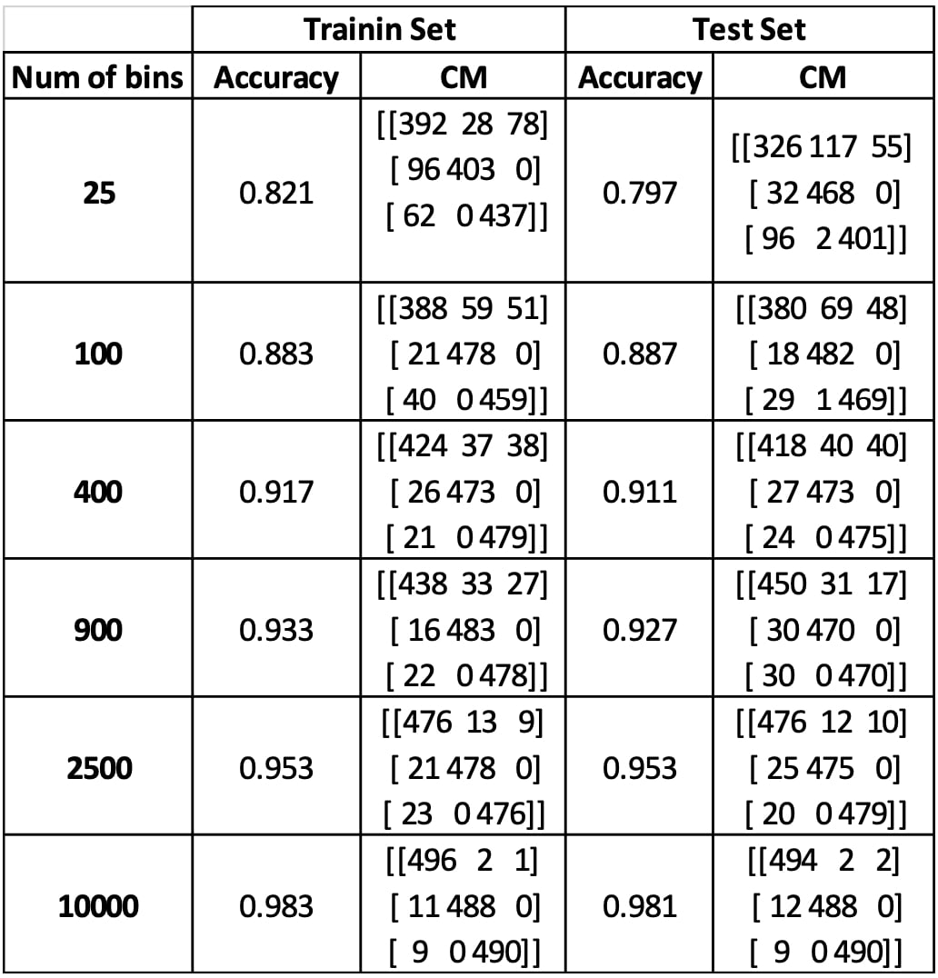
Discussion on Histogram-based Models:

As shown in table 1, increasing the bin number usually results in higher accuracies. This is because when bin number is increased, the grid fitted on the data get into a higher resolution. That way, each cell becomes more reliable representing the data intensity at each portion on the data grid, so that the Bayesian classifier can learn better this representation on the histogram. In conclusion, more bins usually mean more accuracy, but also more computational time. Therefore, one should keep in mind to treat this trade-off optimally according to the application.