Genetic Algorithm for Cost Sensitive Learning
Task
Design and implement a genetic algorithm based approach for cost sensitive learning, in which the misclassification cost is considered together with the cost of feature extraction.
What I have done in brief: I have implemented a genetic algorithm from sctrach, in order to keep the feature extraction cost as minimum as possible while not much comprimising on the classification accuracy. One of the main challanges in this project was to perform a multi-class classification on a highly imbalanced dataset. There are in total 21 features each comes with its own cost if used for classification. The most critical part of this task was formulating the fitness function that would guide the genetic algorithm. So I have defined a fitness function which aims to suppress the feature extraction cost while increasing the class-based accuracies and the overall accuracy. As the classifier, I have employed SVM due its deterministic characteristic that later helped me to fine-tune my fitness function.
Details of the Dataset
The algorithm will be implemented for Thyroid dataset from the UCI repository.
Characteristics:
- Contains separate training and test sets
- The training set contains 3772 instances and the test set contains 3438 instances
- There are a total of 3 classes
- Highly imbalanced train set. Ratios: $\text{Class}_1 \simeq 1\%$ $\text{Class}_2 \simeq 8\%$ $\text{Class}_3 \simeq 91\%$
- In the data lines, each line correspond to an instance that has 21 features and 1 class label
- Data consist of 15 binary and 6 continuous features
- The 21st feature is defined using the 19th and 20th features, which means you don't need to pay for this feature if the 19th and 20th features have already been extracted
- The cost of each feature is given in a seperate file. It does not include the cost of 21st feature since it is a combination of the other features
Steps Followed
- Select a classification algorithm to start with
- Use a bit string representation to indicate what features are selected
- Write an appropriate fitness function that guides the algorithm. This function will include both misclassification cost and the cost of extracting the selected features
Representation of Features:
In order to represent the presence or absence of each feature, I used a bit string which had a length of 21, number of all features. For instance, the following DNA sample represents the presence of second and last three features, while the rest remains absent: 010000000000000000111.
How Did I Formulate the Fitness Function?
Choosing a fitness function is the most critical part of the genetic algorithms and requires every objective and constraint to be taken into account.
So the requirements and constraints I had to watch out can be listed as below:
- A certain subset of features must be selected such that providing a reasonable classification accuracy as well as the minimum possible feature extraction cost
- Class-based accuracy scores should be over a certain limit. This is especially important when we have such an imbalanced multi-class dataset. You might for example reach up to 91% overall accuracy on this specific train set whether you classify all the samples into $\text{Class}_3$
- Decent overall classification accuracy -obviously-
My approach:
First, I focused on handling the imbalance in dataset by somehow parameterizing it in the fitness function. Instead of using the overall accuracy score, I had utilized F-beta score to emphasize more on class-specific accuracies and get more reliable evaluation scores.
As noted above, $F_\beta$ score is the weighted harmonic mean of precision and recall, reaching its optimal value at 1 and its worst value at 0. The parameter $\beta$ determines the weight of precision in the combined score. Therefore $\beta < 1$ assigns more importance to precision, while $\beta > 1$ favors recall. I emphasized Recall by assigning $\beta=1.5$ for this classification task, assigning more importance to classification accuracy of the minority classes. So the first fitness function I came up with was using the $F_\beta$ inversely proportional to the feature extraction cost:
Note that the interval of values $F_\beta$ and $\sum(\text{feature costs)}$ can take quite differ in scale:
$F_\beta: [0,\dots,1]$
$\sum(\text{feature costs)}: [0,\dots,102.3]$
It is explained in the following paragraph why this is NOT good.
The idea was simply to get a higher fitness value when $F_\beta$ score is increased while the feature extraction cost stays lower. Even though the function makes sense, the classifier ended up classifying all instances into $\text{class}_3$ (majority). I figured it out after some further brain-storming why this function wouldn't work as expected. The reason was simply the scale of change in $F_\beta$ scores was not compared to the scale of change in feature extraction cost. Meaning, $F_\beta$ score had a negligible effect on fitness score so that class-based accuracies were not paid attention as intended. $F_\beta$ can take values between 0 and 1, whereas the total selected feature cost varies between a minimum of 0 -meaning no features- and a maximum of 102.3 -cost of selecting all features-. In order to tackle this problem, I introduced a proper modification to this base formula and my final fitness function has finally transformed into:
Multiplying the $F_\beta$ score by seven has been chosen experimentally to make its change more effective in the fitness value. I also used exponential function to further enhance the effect of relatively small improvements in the higher accuracy intervals. In other words, improving accuracy in the 85%~100% range yields more rewards compared to an improvement in the <85% interval.
All in all, the overall range of my fitness value has become: $[0.01,\dots,1097]$. So the fitness value 1097 means that the genetic algorithm found a perfect trade-off, a combination of features that is sufficient to achieve high class-based accuracies while keeping the total feature extraction cost at minimum. We will evaluate the algorithm in each generation by comparing the fitness score it returns to our fitness score range. Notice that this evaluation cannot be thought as similar with the classification accuracy evaluation. What I mean is that reaching to the maximum fitness score 1097 probably means that 1 or 2 lowest cost features are selected out of 21 and yet classifier performed extraordinarily in terms of the class-based accuracies where the lowest is $\approx98\%$. This is of course imposibble most of the times in real life, therefore a more realistic range of the fitness value will be clearer during the training. Consequently, it is not only we are successful when we hit the maximum fitness score but a good trade-off between feature extraction cost and classification accuracy is captured since this is the ultimate purpose.
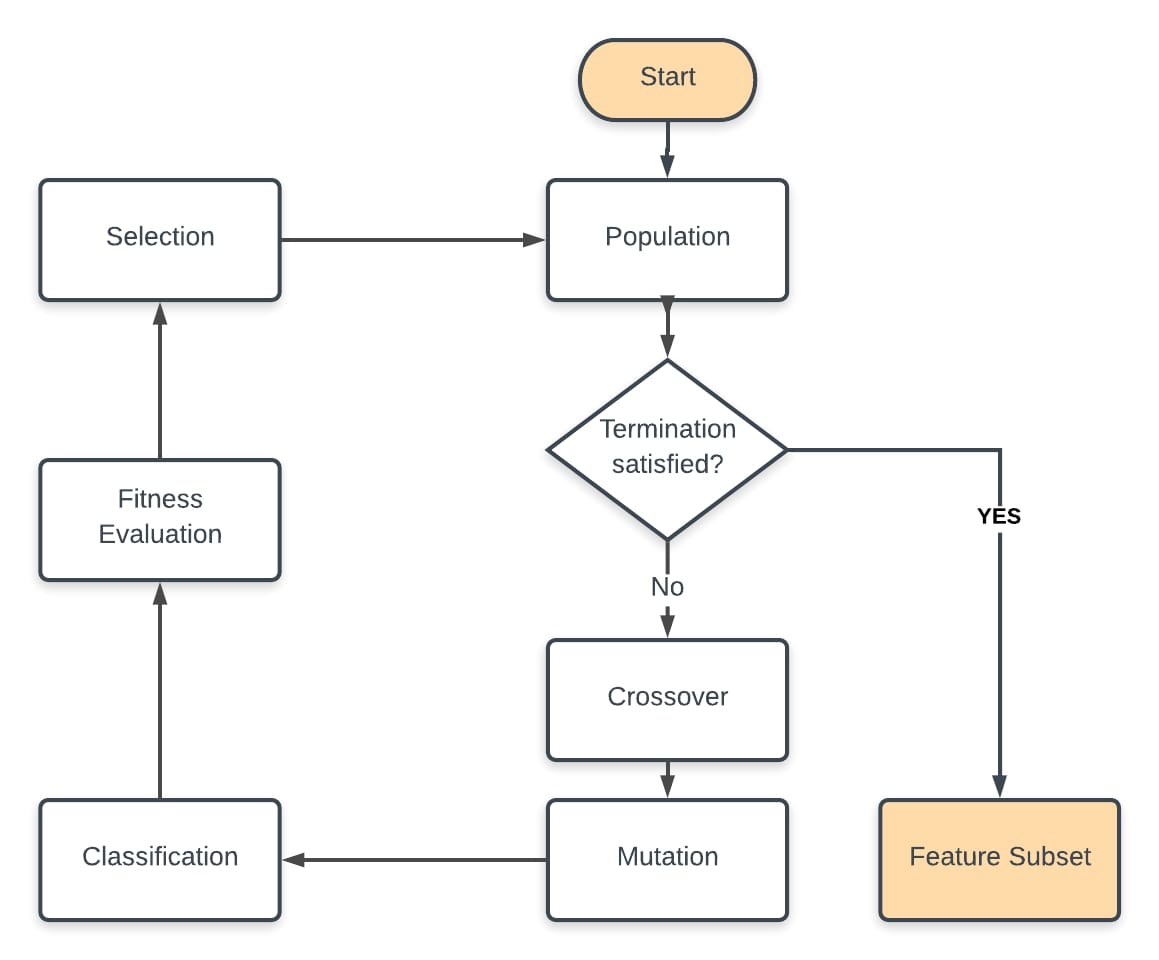
Pseudocode & Flow-Chart
After determining the fitness function and the encoding scheme (bit representation for each feature):
- Randomly Initialize the population
- Perform classification with features selected by the initial population
- Compute the F-beta score and the total feature cost for each DNA in population
- Evaluate the fitness of DNAs using the F-beta score and total cost
- Perform genetic operations selection, crossover and mutation if stopping criterion is not satisfied
- Repeat steps 2 to 5 until a subset of features provides the following gains:
- less than 75% of total feature cost
- minimum 70% class-based f-beta score
- minimum 85% overall f-beta score
- OR the number of generations reach a predetermined threshold.
Classifier: Support Vector Machine
Parameters used:
$C = 6$, $\text{kernel} = \text{‘linear’}$, $\text{gamma} = \text{‘auto’}$, $\text{class_weights} = {\text{class1}: 97.5, \text{class2}: 94.9, \text{class3}: 7.5}$
The reason I chose SVM as the classifier because of its decent performance in higher-dimensions, simplicity, and versatility where different kernels can be easily adapted for decision functions. Moreover, to beat the problem of having a imbalanced dataset even further, I assigned special penalty coefficients to each class for suppressing the misclassification of minority classes. To this end, I calculated the class occurrence frequencies from the training set, and then determined their penalty values between 0-100 inversely proportional to these frequencies. Thanks to these specific penalty values, I was able to benefit from the fastest ‘linear’ kernel achieving over 94% class-based accuracy. Gamma value ‘auto’ is equal to $\frac{1}{n_\text{features}}$. While default value of overall penalty value C is 1, I experimentally set it to 6 to obtain greater class-based and overall classification accuracies.
Genetic Operators and Parameters
Selection
Parameter: $r = 0.4$, where $\text{selection ratio} = 1 - \frac{r}{p}$
These DNAs remain in the next generation. Roulette-wheel selection method is employed.
Cross-over
Parameter: $\frac{r \cdot p}{2}$ many pairs are selected for crossing-over.
They are probabilistically crossed-over and added to the next generation. Mask used for cross-over: 111000111000111000111
Mutation
Parameter: $m = 0.3$, where $\text{mutation ratio} = m \cdot p$
They are selected from the next generation obtained in result of above genetic operations. Point mutation is used.
Number of Population: 6
Number of Generations: 21
Code
import numpy as np
import matplotlib.pyplot as plt
from sklearn import svm
from sklearn.preprocessing import normalize
from sklearn.metrics import confusion_matrix, accuracy_score, fbeta_score
class Genetic:
    def __init__(self, num_population, num_generations, prob_mutation=0.4, survive_ratio=0.5):

        self.num_population = num_population
        self.num_generations = num_generations
        self.prob_mutation = prob_mutation
        self.survive_ratio = survive_ratio
        self.num_survive = 0

        self.population = np.zeros((self.num_population, 21), dtype=np.int)
        self.fitness_values = []

    def init_population(self):
        """
        Initialize a random population.
        :return:
        """

        for i in range(self.num_population):
            individual = np.random.randint(2, size=21)
            self.population[i] += individual
        return self.population

    def selected_features(self, dna, train_x, test_x):
        """
        Return a training set that has features selected by the respective DNA.
        :return: A list that stores features determined by each dna
        """

        selected_features_train = train_x[:, np.argwhere(dna == 1)]
        selected_features_train = np.squeeze(selected_features_train)
        selected_features_test = test_x[:, np.argwhere(dna == 1)]
        selected_features_test = np.squeeze(selected_features_test)

        return selected_features_train, selected_features_test

    def fitness(self, fbeta, feature_cost_list, dna):
        """
        Return a list of fitness values with respect to each DNA.
        :param fbeta_scores: F_beta score of svm classifier that uses certain features selected by the respective DNA.
        :param feature_cost_list: Feature costs are taken into account for cost sensitive learning.
        :param population: Matrix of current population.
        :return: Fitness values of each DNA in the population.
        """

        subtract_cost = 0
        feat_cost = 0

        if dna[-1] == 1:
            if dna[-2] == 1 and dna[-3] == 0:
                subtract_cost += feature_cost_list[-2]
            elif dna[-2] == 0 and dna[-3] == 1:
                subtract_cost += feature_cost_list[-3]
            elif dna[-2] == 0 and dna[-3] == 0:
                subtract_cost = 0

        feat_cost += np.sum(feature_cost_list[np.argwhere(dna == 1)]) - subtract_cost
        #feat_cost = feat_cost/np.sum(feature_cost_list)  # Normalize feature cost

        fitness_val = np.exp(fbeta*7) / feat_cost
        return fitness_val


    def crossover(self, population, fit_val):
        """
        Cross-over the survived genes.
        Mask used: 111000111000111000111
        :param population:
        :return:
        """
        # print('Crossover method-------------')
        num_pop_to_crossover = int(np.round(self.num_population-self.num_survive))#*(1-self.survive_ratio)))

        if num_pop_to_crossover % 2 == 1:
            num_pop_to_crossover -= 1


        selection_prob = np.squeeze(fit_val / np.sum(fit_val))
        # print('crossover selection probs: \n', selection_prob)
        crossover_idx = np.random.choice(len(population), num_pop_to_crossover, replace=False, p=selection_prob)
        # print('Crossover olmaya secilen idx: ', crossover_idx)
        crossover_population = population[crossover_idx, :]

        # print('Pop to be crossover:\n', crossover_population)

        if num_pop_to_crossover % 2 == 1:
            print('Warning! Odd number of genes to crossover!')

        crossed_gen = []

        for i in range(0, len(crossover_population), 2):
            offspring1 = np.concatenate((crossover_population[i][:3],
                                         crossover_population[i+1][3:6],
                                         crossover_population[i][6:9],
                                         crossover_population[i+1][9:12],
                                         crossover_population[i][12:15],
                                         crossover_population[i+1][15:18],
                                         crossover_population[i][18:21]))

            offspring2 = np.concatenate((crossover_population[i+1][:3],
                                         crossover_population[i][3:6],
                                         crossover_population[i+1][6:9],
                                         crossover_population[i][9:12],
                                         crossover_population[i+1][12:15],
                                         crossover_population[i][15:18],
                                         crossover_population[i+1][18:21]))

            crossed_gen.append(offspring1)
            crossed_gen.append(offspring2)

            return np.array(crossed_gen)

    def mutate(self, evolved_population):
        """
        Point mutation used.
        :param evolved_population: Crossovered population.
        :return: Next generation that has mutated random individuals.
        """
        # print('Mutate method----------')
        mutated_gen = []
        # DNA selection to be mutated can be improved by selecting DNAs whose fitness values are lower.
        num_pop_to_mutate = int(np.round(self.num_population*self.prob_mutation))

        if num_pop_to_mutate == 0:
            return evolved_population

        mutate_idx = np.random.choice(len(evolved_population), num_pop_to_mutate, replace=False)
        # print('IDX to mutate: ', mutate_idx)
        mutate_dnas = evolved_population[mutate_idx, :]
        # print('dnas to be mutated:\n', mutate_dnas)

        # Mutate a random bit of each dna in selected portion of population (m.p individuals).
        current_dna_idx = 0
        for dna in mutate_dnas:
            mutate_bit_idx = np.random.randint(len(dna))
            # print('MUTATE BIT: ', mutate_bit_idx)
            dna[mutate_bit_idx] = np.bitwise_xor(dna[mutate_bit_idx], 1)
            evolved_population[mutate_idx[current_dna_idx]] = dna
            current_dna_idx += 1

        return evolved_population

    def next_generation(self, population, fit_val):
        """
        Next generation is selected probabilistically, with higher probability as higher fitness values.
        """
        # print('Next generation method----------')
        # fit_val = np.array(self.fitness_values)
        num_survive = int(np.round(self.num_population*self.survive_ratio))
        self.num_survive = num_survive

        if num_survive % 2 == 1:
            num_survive += 1

        selection_prob = np.squeeze(fit_val / np.sum(fit_val))
        # print('Selection probs: \n', selection_prob)
        # print('sum of probs: ', np.sum(selection_prob))
        # print('POPULATION: \n', population)
        # print('popsize: {}, prob: {}, and its size: {}'.format(population.shape[0], selection_prob, selection_prob.size))
        survive_idx = np.random.choice(population.shape[0], num_survive, replace=False, p=selection_prob)
        # print('survive idx: ', survive_idx)

        #next_generation = self.population[next_gen_idx, :]
        survived_dnas = population[survive_idx, :]

        return survived_dnas


def evaluate(true_labels, predicted, cm=True):
    """
    Evaluate the classifier.
    :param true_labels:
    :param predicted:
    :param cm:
    :return:
    """

    accuracy = np.round(accuracy_score(true_labels, predicted), decimals=3)
    if cm is False:
        return accuracy
    else:
        cm = confusion_matrix(true_labels, predicted)
        cls_based_accuracies = cm.astype('float') / cm.sum(axis=1)[:, np.newaxis]
        cls_based_accuracies = np.round(cls_based_accuracies.diagonal(), decimals=3)
        return accuracy, cm, cls_based_accuracies

def calc_weighted_costs(Y):
    """
    Since thyroid dataset is quite imbalanced, assigning special weights to
    classes gives more accurate class-based classification performance.
    :param Y: train or test labels.
    :return: penalty weights of each class for SVM classification.
    """
    num_samples_cls3 = np.count_nonzero(np.argwhere(Y == 3))
    num_samples_cls2 = np.count_nonzero(np.argwhere(Y == 2))
    num_samples_cls1 = np.count_nonzero(np.argwhere(Y == 1))

    cls1_weight = (num_samples_cls2+num_samples_cls3) / (num_samples_cls1+num_samples_cls2+num_samples_cls3)
    cls2_weight = (num_samples_cls1+num_samples_cls3) / (num_samples_cls1+num_samples_cls2+num_samples_cls3)
    cls3_weight = (num_samples_cls1+num_samples_cls2) / (num_samples_cls1+num_samples_cls2+num_samples_cls3)
    return cls1_weight*100, cls2_weight*100, cls3_weight*100


def run_genetic(genetic_config, wclf):

    population = genetic_config.init_population()
    #print('Initial population:\n', population)

    fit_vals = np.zeros((genetic_config.num_population, 1))
    fittest_value_record = np.zeros((genetic_config.num_generations, 1))

    fbeta_vals = np.zeros((genetic_config.num_population, 1))
    fittest_fbeta_record = np.zeros((genetic_config.num_generations, 1))

    cls_bsd_rec = []
    best_dna_record = np.zeros((genetic_config.num_generations, 21), dtype=np.int)
    best_acc_dna = []

    for i in range(genetic_config.num_generations):
        print('GENERATION: {} ------------------------------'.format(i))
        print('Population:\n', population)

        # HERE TRAIN SVM ACC. TO SELECTED FEATURES
        # PASS F1 SCORES FOR EACH SVM TRAINED ON FEATURES THAT ARE SELECTED BY DNAs.
        for j in range(genetic_config.num_population):
            selected_x_train, selected_x_test = genetic_config.selected_features(population[j], train_x, test_x)
            # selected_x_train = normalize(selected_x_train)
            # selected_x_test = normalize(selected_x_test)

            wclf.fit(selected_x_train, train_y)

            predicted = wclf.predict(selected_x_train)
            print('PREDICTED includes: ', np.unique(predicted))
            #print('Test_Y includes: ', np.unique(train_y))

            f_beta = fbeta_score(train_y, predicted, beta=1.1, average='weighted')
            fbeta_vals[j] += f_beta

            acc, cm, cls_based = evaluate(train_y, predicted)
            cls_bsd_rec.append(cls_based)

            if np.min(cls_based) > 0.83:
                best_acc_dna.append(population[j])
                print('Good DNA recorded. Index: ', len(cls_bsd_rec)-1)

            # class_based_acc_record[j] += cls_based
            # print('DNA{} F_beta score: {}'.format(j, f_beta))

            fitness_val = genetic_config.fitness(f_beta, feature_costs, population[j])
            # print('DNA{} fitness: {}'.format(j, fitness_val))
            fit_vals[j] += fitness_val

        fittest_value_record[i] += np.max(fit_vals)
        fittest_fbeta_record[i] += fbeta_vals[np.argmax(fit_vals)]
        best_dna_record[i] += population[np.argmax(fit_vals)]

        print('\nFittest value: ', fittest_value_record[i])
        print('Fittest FBETA value: {}\n'.format(fittest_fbeta_record[i]))
        # print('Fittest Class-based acc: ', class_based_acc_record[np.argmax(fit_vals)])

        # Create new generation
        survived_dna = genetic_config.next_generation(population, fit_vals)
        # print('direct Next GEN: \n', survived_dna)
        crossed_dna = genetic_config.crossover(population, fit_vals)
        # print('Crossed:\n', crossed_dna)
        next_gen = np.concatenate((survived_dna, crossed_dna), axis=0)
        # cp_next = np.copy(next_gen)
        # print('NEXT GEN: \n', next_gen)
        next_gen = genetic_config.mutate(next_gen)
        # print('NEXT GEN: \n', next_gen)
        population = next_gen

        if i == genetic_config.num_generations-1:
            last_best_idx = np.argmax(fit_vals)
        # Zero-out fitness values for the new generation.
        fit_vals = np.zeros((gen.num_population, 1))
        fbeta_vals = np.zeros((gen.num_population, 1))

    return fittest_value_record, fittest_fbeta_record, best_dna_record,
            cls_bsd_rec, last_best_idx, population, best_acc_dna
# Load the dataset
train_x = np.loadtxt('./cs550_data/ann-train.txt')[:, :-1]
train_y = np.loadtxt('./cs550_data/ann-train.txt')[:, -1].astype(int)
test_x = np.loadtxt('./cs550_data/ann-test.txt')[:, :-1]
test_y = np.loadtxt('./cs550_data/ann-test.txt')[:, -1].astype(int)

# These are pre-known costs of each feature available
feature_costs = np.array([1.0, 1.0, 1.0, 1.0, 1.0, 1.0, 1.0, 1.0, 1.0, 1.0, 1.0,
                          1.0, 1.0, 1.0, 1.0, 1.0, 22.78, 11.41, 14.51, 11.41, 25.92])


#%% CLASSIFIER: class-weighted SVM

cls1_w, cls2_w, cls3_w = calc_weighted_costs(train_y)

# Fit and train the model using weighted classes
wclf = svm.SVC(C=6, kernel='linear', gamma='auto', class_weight={1: cls1_w, 2: cls2_w, 3: cls3_w})

#%% GENETIC Feature Selector
gen = Genetic(num_population=6, num_generations=21, prob_mutation=0.3, survive_ratio=0.4)
fittest_values, fbeta_record, best_dnas, \
class_based_acc_record, last_best_dna_idx, last_generation, best_acc_dna = run_genetic(gen, wclf)

print('Last Generation: \n', last_generation)
print('Last best dna index: ', last_best_dna_idx)
print('Fittest Vals:\n{}'.format(fittest_values))
print('Fbeta Scores: \n{}'.format(fbeta_record))
print('Last best class-based acc: ', class_based_acc_record[-gen.num_population:][last_best_dna_idx])

plt.plot(fittest_values)
plt.ylabel('Fitness')
plt.xlabel('Generation')
plt.title('Fittest Value per Generation')
plt.show()

plt.plot(fbeta_record)
plt.ylabel('Fbeta')
plt.xlabel('Generation')
plt.title('Fbeta Score per Generation')
plt.show()

class_based_acc_record = np.array(class_based_acc_record)
x = np.arange(len(class_based_acc_record))
yc1 = class_based_acc_record[:,0]
yc2 = class_based_acc_record[:,1]
yc3 = class_based_acc_record[:,2]
y_array = np.array([yc1, yc2, yc3])
labels = ['class1', 'class2', 'class3']

for y_arr, label in zip(y_array, labels):
    plt.plot(x, y_arr, label=label)

plt.legend()
plt.title('Class-based Fbeta Scores')
plt.xlabel('DNAs (all generations)')
plt.ylabel('Fbeta Score')
plt.show()
Results
After constructing the SVM classifier with the mentioned parameters, I ran the genetic algorithm on train set to select features wisely. At the end, I obtained last generation’s fittest DNA -representing the selected features-, and have the classifier perform predictions on test set using this feature subset determined by the DNA. Results are reported below:
Fittest DNA of Last Generation and Selected Features:
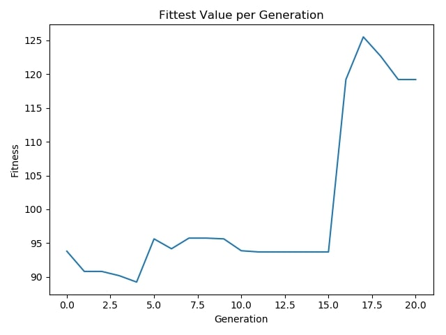
111001100010010111000 with the fitness score: 119.19
[age, sex, on_thyroxine, sick, pregnant, query_hyperthyroid, hypopituitary, psych, TSH, T3]
Total Cost of Selected Features:
$1+1+1+1+1+1+1+1+22.78+11.41 = 42.19$
Train Set Results:
$\text{Class-based accuracies}: [0.794 0.958 0.986]$
$F_\beta: 0.94$
Test Set Results and Graphs:
$\text{Overall accuracy}: 0.971$
$\text{Class-based}: [0.709, 0.96 , 0.978]$
$ \text{Confusion matrix} = \begin{bmatrix} 51 & 22 & 0 \\ 7 & 170 & 0 \\ 18 & 53 & 3107 \end{bmatrix}$
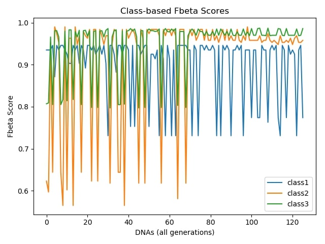
Class-based Accuracies During Evolution:
Fittest Value per Generation:
Conclusion
Employing a genetic algorithm in this task helped me to select which features were crucial to perform a decent cost-sensitive classification. This can especially be useful in situations which we cannot use all of the features due to some constraints such as lack of hardware resources or when the cost of feature extraction matters drastically. This approach is also helpful in cases when we don't have any prior knowledge on features and should take care of the constraints mentioned above.
As shown in the results, we have managed to select the most beneficial subset of features. The algorithm selected 10 features out of 21, costing 42.19 in total, therefore earns us $102.3-42.19 = 60.11$ which is less than half the price compared to the case where all the features are utilized. Moreover, we can say the classifier has performed well on test set observing the class-based accuracies. Besides hitting satisfactory accuracies on relatively major classes, it was capable of reaching up to 70% accuracy for the very minority class which had less than 1% of samples in the dataset. On the other hand, graphs demonstrate how the algorithm performs on the way to the final result. They make perfect sense picturing the unstable nature of genetic algorithms, as they are inspired by the evolution and natural selection phenomenon so that the randomness always plays role in each iteration. Therefore they usually oscillates in terms of fitness of the objectives up to the final results.