Clustering
Task: Given an image, cluster image pixels using partitional and hierarchical clustering algorithms.
In this project I have implemented k-means and agglomerative clustering algorithms. You will find brief explanations of my code throughout the implementation.
K-means
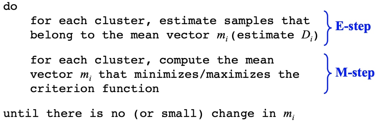
K-means is basically an example of the Expectation-Maximization algorithm. Mainly, starting with randomly initialized cluster (mean) vectors mi, we loop through:
I used Mean Squared Error as my distance metric to evaluate pixel clusters in each iteration. Each cluster is represented with a mean vector, also called a centroid. Experimented with different k values and chose the optimal one using the elbow method.
Code
Let's import the necessary libraries.
import numpy as np
import scipy.io
import imageio
import pylab
import time
import matplotlib.pyplot as plt
from PIL import Image
I've created a class called Kmeans in order to have all the functionalities clean and neat. All the methods are explained as docstrings and comments in the code.
class Kmeans:
    def __init__(self, k):
        self.K = k
        self.num_of_K = len(k)
        self.all_error = []


    def init_rand_centroids(self, im, num_clusters):
        """ Initialize centroids as random pixels in the image. Returns k-many random pixel RGB coordinates.

        Steps in this method:

        1. Create a 1-d numpy array that represents the indexes of each individual pixel in the input image
        2. Shuffle the array
        3. Use the shuffled array as a mask to obtain randomly selected centroids
        4. Return the RGB values of the selected centroids
        """

        initial_points = np.arange(im.shape[0])
        np.random.shuffle(initial_points)
        centroid_locs = im[initial_points[:num_clusters], :]
        return centroid_locs


    def update_centroids(self, mse, k, labels):
        """ Returns new centroids using the current labeling of the pixels and the corresponding overall MSE.
        """
        current_centroid = np.zeros((k, 3))
        error = 0
        for i in range(k):
            indexes = np.where(labels == i)[0]  # Indexes of pixel labels where they belong to ith cluster.
            if len(indexes) != 0:
                values = im2[indexes, :]  # Get the RGB values of the pixels using their indexes as mask.
                current_centroid[i, :] = np.mean(values, axis=0)  # Compute the mean of the new centroid.
                # Calculate MSE for the updated centroids.
                error += np.sum((values[:, 0] - current_centroid[i, 0]).astype(np.float64) ** 2 +
                                (values[:, 1] - current_centroid[i, 1]).astype(np.float64) ** 2 +
                                (values[:, 2] - current_centroid[i, 2]).astype(np.float64) ** 2)
        mse += error / len(labels)
        return current_centroid, mse

    def predict(self, k, new_im):
        """ Return current labels of pixels, updated centroids, and corresponding MSE.
        """

        # Select random centroids.
        centroids = self.init_rand_centroids(new_im, k)

        iteration = 0
        mse = 0

        # Compute distances of pixels to randomly selected centroids before the while loop as the first step.
        dist = np.zeros((im2.shape[0], k))  # Distance matrix for each pixel.
        for i in range(k):
            dist[:, i] = np.linalg.norm(im2 - centroids[i], axis=1)  # This calculates the Euclidean distance.
        labels = np.argmin(dist, axis=1)  # Assign each pixel to a cluster, which is the closest one.
        centroids, mse = self.update_centroids(mse, k, labels)

        # Repeat the above process until any pixels didn't change their labels.
        while not (labels == np.argmin(dist, axis=1)).all():

            if iteration != 0:
                dist = np.zeros((im2.shape[0], k))
                dist[:, i] = np.linalg.norm(im2 - centroids[i], axis=1)
                labels = np.argmin(dist, axis=1)

            centroids, mse = self.update_centroids(mse, k, labels)
            iteration += 1

        return labels, centroids, mse


    def fit(self, im, im2):
        """ Outputs the clustered image for each value of k.

        im: Original image, of size (1000, 1600, 3) in this case.
        im2: Reshaped image array from 3d to 2d. Thus in size (1600000, 3)
        """
        clustered = np.zeros((self.num_of_K, im.shape[0], im.shape[1], 3), dtype=np.uint8)
        err = []

        # This loop is to run k-means algorithm for different given values of k.
        # So it will run k-means algorithm as many as number of the k values provided (num_of_K).
        for k in range(self.num_of_K):
            print("Computing for K =", self.K[k])

            labels, centroids, mse = self.predict(self.K[k], im2)
            err.append(mse)  # Save mse values to plot them later.
            labels = labels.reshape((im.shape[0], im.shape[1])).T  # Reshape label matrix back to original image dimensions.
            clustered_im = np.zeros((im.shape[0], im.shape[1], 3), dtype=np.uint8)

            # Re-construct the image with the final clustered pixels.
            for i in range(im.shape[0]):
                for j in range(im.shape[1]):
                    clustered_im[i, j, :] = centroids[labels[j, i], :].astype(np.uint8)

            # Save clustered images for different k values to plot.
            clustered[k, :, :, :] = clustered_im

            print("Mean Squared Error = ", np.round(mse, decimals=2))
            # Print centroids for k values smaller than 16 to prevent the longer output.
            if self.K[k] <= 16:
                print("Centroids =\n", np.around(centroids).astype(int))
            print("------------------------")

        # Plot the clustered images and the progressive MSE value.
        for i in range(self.num_of_K):
            plt.figure()
            pylab.imshow(clustered[i, :, :, :])
            pylab.title("K: {}".format(self.K[i]))

            self.all_error.append(np.round(err[i], decimals=2))

        plt.figure()
        plt.plot(self.K, self.all_error)
        plt.xlabel("K value")
        plt.ylabel("Mean Squared Error")
        plt.show()
Now we can read the image and run the algorithm with different k values. Centroid vectors, mean squared errors and the resulting images after clustering are reported in the output. As an example, I used k values (2, 4, 8, 16, 32, 64, 128).
#%% Main

# Read the image.
im = imageio.imread('./sample.jpg')

# Plot the original image.
plt.figure()
pylab.imshow(im)
pylab.title("Original Image")
plt.show()

# Convert to np array and reshape to work in 2d.
im = np.array(im)
im2 = im.reshape(-1, 3)
print('\nImage shape: {}.\n'.format(im.shape))

# Run k-means for the following k values.
K = (2, 4, 8, 16, 32, 64, 128)

start_time = time.time()

k_means = Kmeans(K)
k_means.fit(im, im2)
print("\nCluster vectors calculated for the K-values: ", K)
print("\nCorresponding MSE values: ", k_means.all_error)
print("\nTime passed: ", np.round((time.time() - start_time), decimals=2), "seconds.")
print("Process finished.")


Take aways
As seen in the output above, the image look more similar to its original as the number of clusters increases. This is quite expected since we tell algorithm to represent the whole input image in only two colors when we set k=2.
On the other hand, according to the experiment results with varying k values, one might simply choose k=32 using the elbow method over mean squared error graph. As this method suggests, one should choose a number of clusters so that adding another cluster doesn't give much better modeling of the data.
Agglomerative
Challange: Computational time for this algorithm will be dramatically higher compared to the k-means algorithm. This is because agglomerative clustering considers each individual sample (pixels in this case) as a different cluster and then computes the (dis)similarity between each of these clusters. Similar clusters are then merged together and that keeps on until the user defined number of clusters are reached at the end. Remember we had always k-many clusters even in the beginning of the k-means algorithm and compared each pixel with the mean of these cluster. This means k(num_pixels) comparisons where on the other hand the number of comparisons are equal to num_pixels2. Note that the greatest k value we used was 128 while number of pixels was 1000×1600=1600000.
Solution: We should somehow form small groups of pixels, instead of counting each pixel as another cluster, and consider them as the initial clusters of the agglomerative algorithm. We might have downsample the image to a lower resolution but a better approach would be using the clusters we already have from the output of the k-means algorithm.
So the agglomerative clustering algorithm:
Let each sample be a cluster
compute the dissimilarity matrix
repeat
merge the two most similar clusters
update the distance matrix
until only a single cluster remains
Code
import numpy as np
import matplotlib.pyplot as plt
import pylab
import imageio
def agglomerative(initial_data, k):

    iterations = 0
    while len(initial_data) != k:

        distance_matrix = np.zeros((len(initial_data), len(initial_data)), dtype=np.double)

        for i in range(initial_data.shape[0]):
            distance_matrix[i] = np.linalg.norm(initial_data - initial_data[i], axis=1)

        # Add 10000 to diagonal to get rid of 0s as the min value in following steps.
        np.fill_diagonal(distance_matrix, 10000)
        # Check diagonal.
        # print(distance_matrix.diagonal())

        # Now get min indices.
        min_index_1, min_index_2 = np.argwhere(distance_matrix == np.min(distance_matrix))[0]
        # print(min_index_1, min_index_2)

        # Merge two cluster vectors. Basically take mean of two vectors.
        mn = np.mean((initial_data[min_index_1], initial_data[min_index_2]), axis=0)
        # Delete merged vectors.
        initial_data = np.delete(initial_data, [min_index_1, min_index_2], 0)
        # Add new mean vector.
        initial_data = np.append(initial_data, np.array([mn]), axis=0)

        iterations += 1

    new_clust_vecs = initial_data
    return new_clust_vecs
#%% Main

im = imageio.imread('./sample.jpg')
# Convert to np array.
im = np.array(im)
im2 = im.reshape(-1, 3)

# Load the output clusters of k-means saved into a text file.
initial_data = np.loadtxt('kmeans_256centroids.txt').astype(np.double)

# There will be 16 clusters left as the output of agglomerative clustering.
k = 16
new_clusters = agglomerative(initial_data, k)

dist = np.zeros((im2.shape[0], k))
for i in range(k):
    dist[:, i] = np.linalg.norm(im2 - new_clusters[i], axis=1)
labels = np.argmin(dist, axis=1)

clustered = np.zeros((k, im.shape[0], im.shape[1], 3), dtype=np.uint8)

print('Final Centroids:\n', new_clusters.astype(int))

# This loop can be scaled up for different k values.
for n in range(1):

    labels = labels.reshape((im.shape[0], im.shape[1])).T

    clustered_im = np.zeros((im.shape[0], im.shape[1], 3), dtype=np.uint8)

    for i in range(im.shape[0]):
        for j in range(im.shape[1]):
            clustered_im[i, j, :] = new_clusters[labels[j, i], :].astype(np.uint8)

    clustered[n, :, :, :] = clustered_im

for i in range(1):

    plt.figure()
    pylab.imshow(clustered[i, :, :, :])
    pylab.title("K: {}".format(k))

Conclusions
To sum up, hierarchical clustering is more flexible and has fewer hidden assumptions than partitional clustering about the distribution of the underlying data. Hence in k-means you should know a bit about cluster numbers priorly or at least have an educated guess. However agglomerative clustering is computationaly costly if you don't form groups of samples before running the algorithm. Choosing one over another truly depends on the specific application. For instance, if there is a prior belief about cluster numbers, k-means gives very satisfactory results.