Estimate the Age of People From Photos with Convolutional Neural Networks
In this project, our task was to design and train a deep age estimation network that will accurately predict age of people, whose ages vary between 1 and 80, from their 91x91 facial grayscale images. Since we were not allowed to use any wrappers like tflearn or keras, we have implemented the convolutional block, residual block and pooling operations from sctrach and designed our own network by using these blocks. As for the dataset, we have used a downsampled subset of UTKFace dataset, provided by the instructor of the course. Significant amount of experiments are conducted all of which are runned on 2 NVIDIA GeForce GTX 1080 Ti using Tensorflow.
While fine-tuning, greedy approach is followed to limit the number of experiments, i.e. once there’s a winner in a current experiment, the following experiments are conducted by fixing the winner configuration for current hyperparameter and changing another hyperparameter in the next experiments one at a time. In our preliminary experiments, we observed that our models converge around 50 epochs and due to high number of experiments, we fixed the number of total epochs to 50 till we apply early stopping scheme. Until further investigation of each hyperparameter, the following initial values are used due to avoid dramatic oscillations in the learning process: batch size is 128, learning rate is 0.001, learning rate decay factor is 0.1, learning rate decay step is 860 (corresponds to 20 epochs), and initializer is Xavier. Note that these parameters are also investigated and fine-tuned in the next steps and are used at the beginning only for stable comparison reasons of our models in the architecture selection step.
1. Architecture Design
We first began by delving into all the possibilities of convolution, pooling, and dense layers and tried various architectures. Our approach was to start experimenting with number of convolution operations and the position of pooling layers between those operations. Therefore, we have created several different architectures, as shown in Table 1, combining the positions of consecutive convolution and pooling operations.
First, we compared models by holding the filter number and filter size the same in terms of their validation mean-absolute-error scores. As an intuitive approach, we generally preferred an increasing number of convolutional filters as we add more convolutions. The reason is that we expect our model to learn more complex representations of the input image as we go deeper, therefore, tried to capture more of these details with higher number of filters. After that, we picked some models that outperformed the rest, considering the MAE score along with the model complexity.
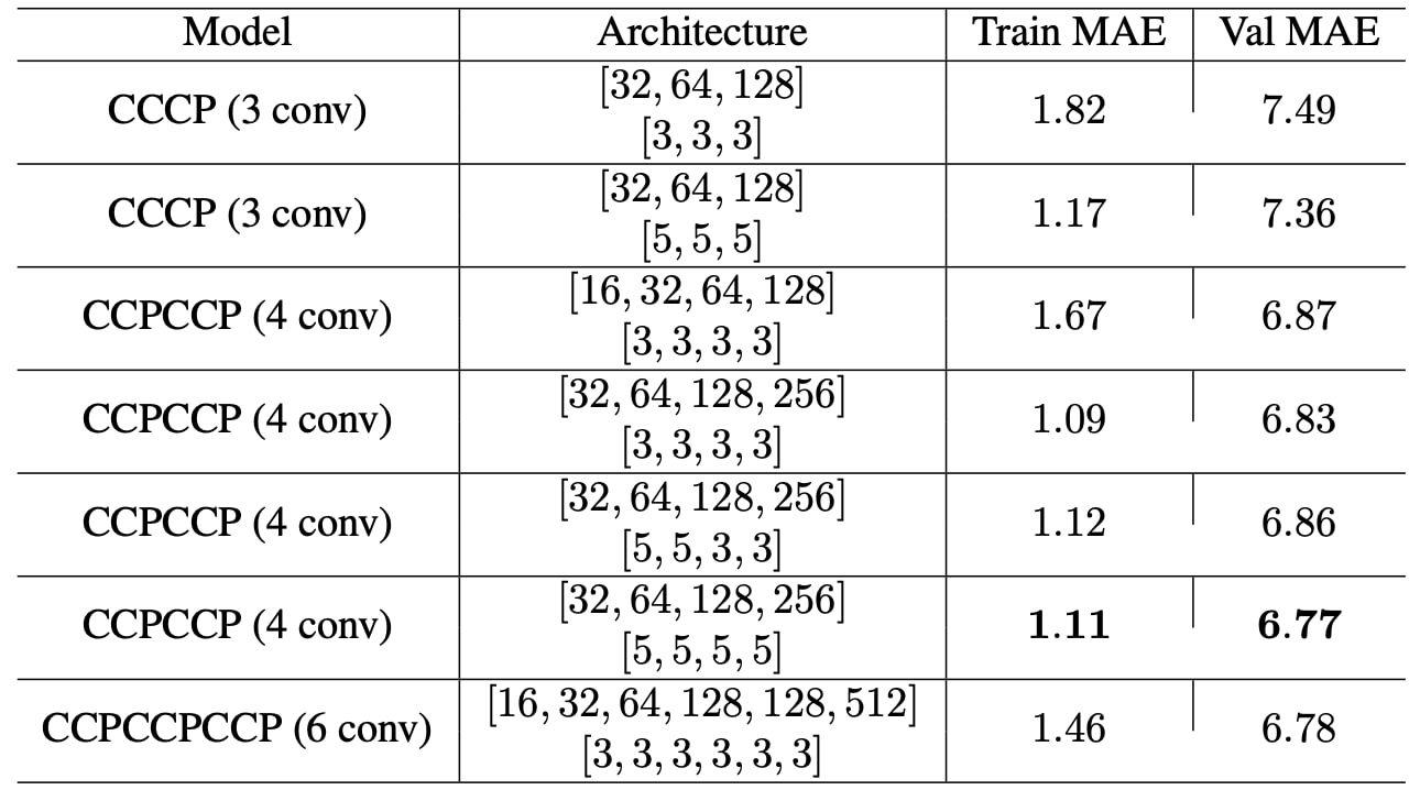
Table 1. Designed convolutional neural network models with their mean-absolute-value results. Letters ’C’ and ’P’ denote ’Conv2d’ and ’MaxPool2d’ operations respectively. All pooling operations are identical as of size 2x2 and stride 2. Number and size of convolutional filter information wrapped in list representations, each element denoting the convolution operation parameters in respective order. For instance, [32,64,128] and [3,3,3] implies there are 3 convolutional operation consisting of 32, 64 and 128 number of filters where each has size 3x3.
Therefore, models with higher complexity but with slightly better MAE scores are also eliminated. Then we have experimented by changing number of filters and their size for the pre-selected models in the previous step. According to our experiment result in this step, models with 4 convolutional blocks generally performed better than the ones which have less or more convolutional operations. Subsequently, we focused our experiments more on this architecture and investigated with further different filter configurations. As a result, we obtained the best parameter selection as with 4 convolutions consisting of filter numbers of 32, 64, 128, and 256, each has filter size of 5x5, corresponding to the sixth row of Table 1.
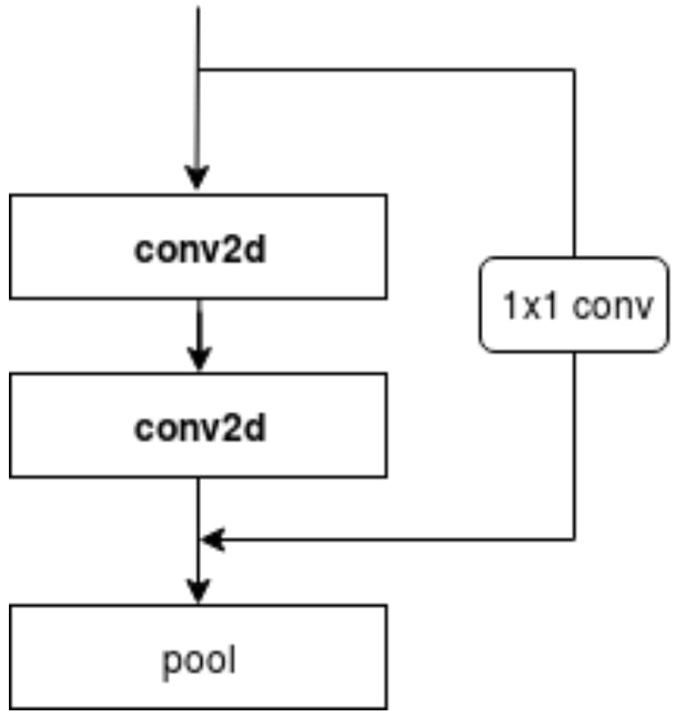
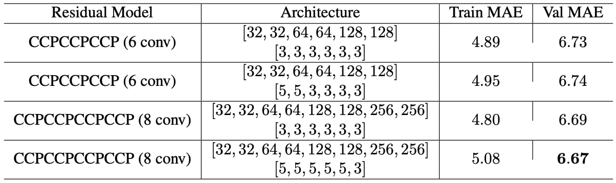
At some point, we observed that deep architectures overfit the training data quite easily; however, they do not convey much of the learned representation to the validation set. This was quite expected since we did not employ any regularization technique during the training period for this step. However, we decided to add residual shortcuts to our convolutional architecture in the hope that it will help the architecture perform better also in validation set when its depth is increased. Following the same architecture selecting approach as we did before, we experimented with even deeper models using residual units shown in Figure 1.
Although we constructed quite deeper models compared to our prior experiments, residual units did not contribute much in our case. Shortcut connections demonstrated some natural regularization behaviour as we can easily see the decrease between train and validation MAE scores shown in Table 2. Even if the models got deeper, overfitting trend was quite reasonable especially compared to the previous models that we experimented. On the other hand, they did not improve the validation MAE scores significantly, while introducing much more complexity as the number of parameters increases as they get deeper.
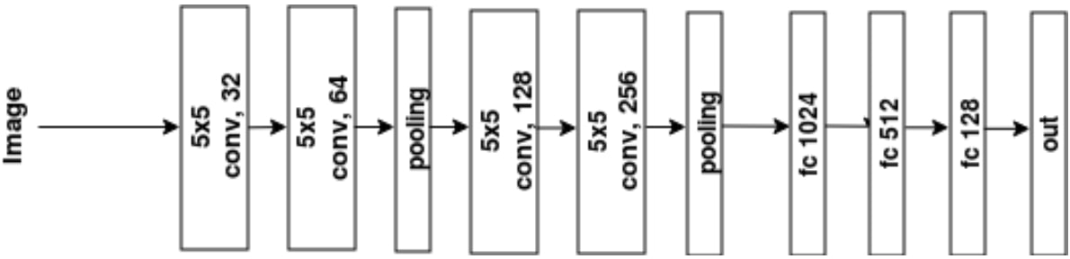
Consequently, we decided to fine-tune the model in Figure 2 with a fairly simple structure and a reasonable initial validation MAE score.
2. Loss Function
We used mean squared error (MSE) for optimization:
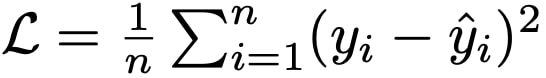
where yi is the ground truth label, ˆyi is the predicted label for sample i, and n is the mini batch size. Although evaluation of the model on both validation and test set are done in terms of mean absolute error (MAE), using MSE during training allows the model to penalize the incorrect predictions more as they get differ a lot from the ground truth.
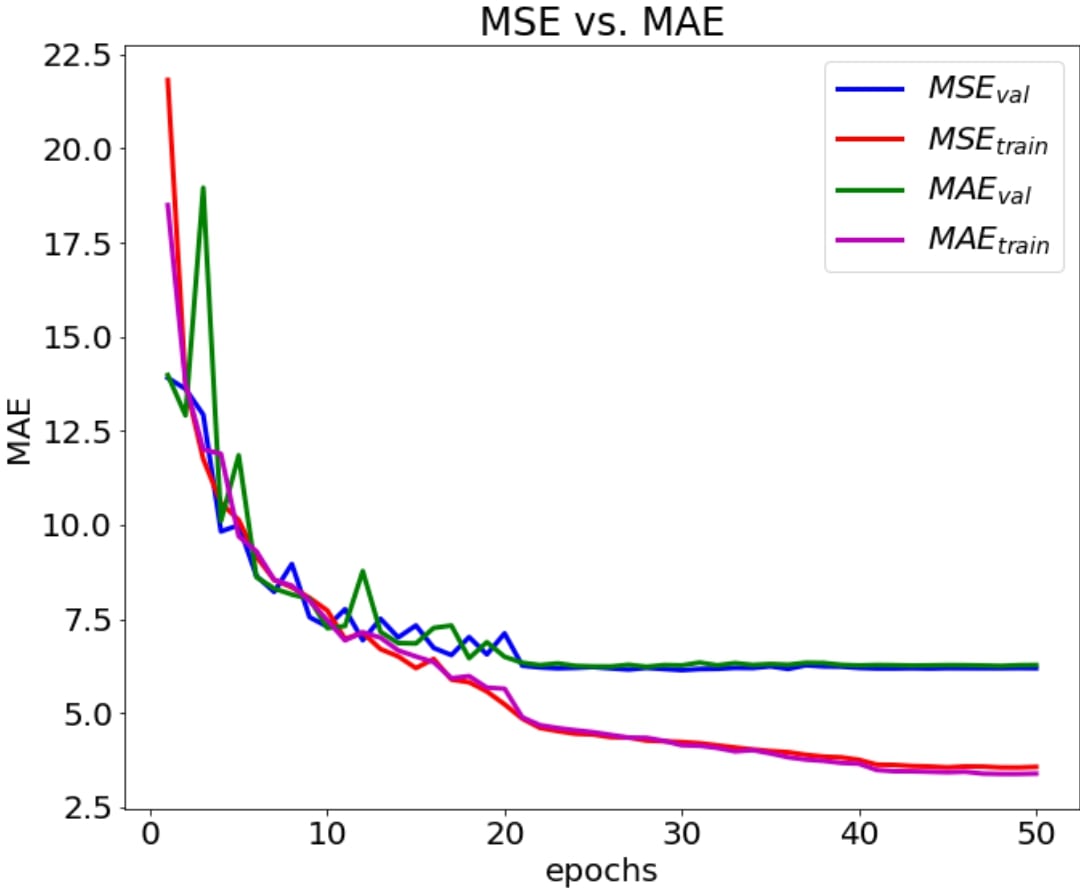
We show the benefit of using MSE by training both with MSE and MAE in Figure 3, where in the case of MAE the network does not perform as good as MSE: its MAE value on validation set (6.19) was slightly inferior to that of MSE (6.28). Please note that, MSE is used only for optimization during training. Throughtout the whole report, all decisions are made by inspecting the validation set MAE value at the end of training.
3. Effect of Initialization
In this chapter, we investigate the effect of Xavier, random normal, and additionally He uniform initialization for the network’s weights and filters. For the random normal initialization, we used tf.initializers.truncated normal rather then tf.initializers.random normal since in the former values more than two standard deviations from the mean are discarded and re-drawn. This is the recommended initializer for neural network weights and filters in Tensorflow.
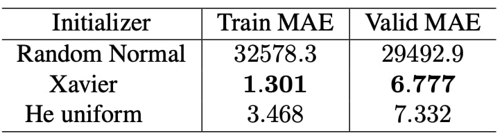
From Table 3, it is seen that initialization with random normal is nonsense because other initialization methods are designed meticulously for deep neural architectures and therefore they perform far superior to random normal. Since He uniform is proposed 5 years after Xavier, we were expecting it to perform better than Xavier. However, this is not the case. Arguably, this may be because of our shallow architecture.
4. Learning Rate
Before further proceeding, we want to make sure that our learning rate is set properly. Therefore, we examined the effect of learning rate which is given in Table 4.
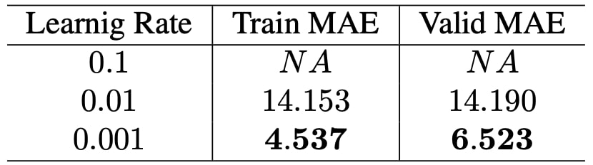
Surprisingly, for learning rate 0.1, optimizer is not able to run. It gave nan as the training loss from the beginning of first epoch. We proceed our experiments by setting learning rate to 0.001 from now on. Note that all the experiments shown in Table 4 are performed using learning rate decay step as 860 which cor- responds to 20 epochs. This value is found by manual inspection.
5. Batch Normalization
Batch normalization (BN) is an effective way to reduce internal covariate shift, which increases the performance of model. Therefore, investigating its effect is a must in deep architecture training. Although applying BN before or after activation function is quite controversial, we followed the order proposed in this paper and applied it before the activation function. Thus, each convolution and dense layers is followed by a BN layer. It enhanced the performance approximately 14% by dropping the validation MAE to 5.856.
6. Regularization
We applied two types of regularization: l2-regularization and dropout. We finetune the dropout probability on each dense layer and then with the best performing configuration, we fine-tune the l2-regularization penalty, i.e. weight decay rate.
6.1. Dropout
Since we have three fully connected layers, our model is prone to overfit the training data. An effective way to prevent this is to use of dropout.
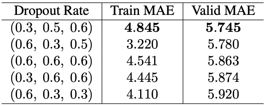
Firstly, we experiment with the same dropout rate for each three dense layer. We applied all dropout rates in the range [0.3, 0.9]. Among these seven option, the best performers are 0.3, 0.5, and 0.6. Then, we applied grid search for each three dense layer with these three values. Table 5 displays the results of top 5 performing rates. Unsurprisingly, high dropout rates perform better than low ones since the network memorize the training data and having high dropout rates forces network to forget some data coming from previous layers. Since (0.3, 0.5, 0.6) performed better than others, we choose it and proceed to next experiments.
6.2. L2-regularization
L2-regularization is not unique to deep learning architectures but it helps a lot by putting a restriction on each filter’s weights so that they are bounded and they are all around same values, i.e. some weights cannot be much higher than the others. We added l2-regularization to each convolution and dense layer. Then the loss function defined in chapter 3 becomes:
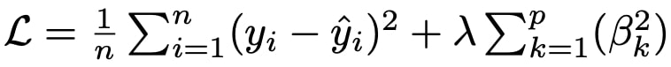
where λ is the weight decay factor, βk is the kth weight matrix, and p is the total number of weight matrices. We try 5 different λ values. Table 6 displays the outcomes.
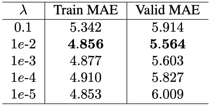
As it can be seen, very high rates degrade both the training and validation performance since it causes model to underfit. On the other hand, very low rates don’t add much to the performance. Usually, 1e−3 or 1e−5 is advised to be used in deep learning frameworks; however, 1e−2 performed the best in our experiments. Therefore, we proceed with it.
7. Optimizer
We use Adam optimizer with default parameters in Tensorflow. We continue our experiments with finetuning batch size. At this point, we also applied early stopping scheme to prevent network overfitting the training data. We think that when batch size is changed and early stopping is applied, the previous best performed learning rate, which was 0.001, may also need to be updated. Therefore, we run the experiments by playing with the learning rate, batch size whilst early stopping scheme is on. Training process is early stopped when last 20 epochs’ validation MAE scores are not improved by 0.2. Inspection window size (20) is chosen in accordance with learning rate decay step. 0.2 is determined by manual inspection of the change of validation MAEs over epochs after saturation. Therefore, we did not fine-tune these parameters again in our experiments. Maximum number of epochs is set to 100. However, all of the experiments are early stopped. Table 7 shows the outcomes of experiments.
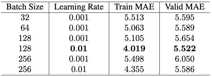
Note that best performing learning rate was initially found as 0.001 in chapter 5; however, it is replaced with 0.01 according to the Table 7. We believe that this because of the combined affect of batch size and early stopping scheme.
8. Test Results
Since we finalized our model selection using validation set, it is now time to test our model on the test set. Our model achieved 4.018 train MAE, 5.522 validation MAE, 5.568 test MAE score.
9. Code
import os
import numpy as np
import tensorflow as tf
import uuid
import mlflow
os.environ['CUDA_VISIBLE_DEVICES'] = '2'
session = tf.Session(config=tf.ConfigProto(gpu_options=tf.GPUOptions(allow_growth = True)))
# session = tf.InteractiveSession(config=tf.ConfigProto(gpu_options=tf.GPUOptions(allow_growth = True)))
MLflow settings
This is to keep track of metrics while the model trains on the GPU server.
experiment_path = 'experiments'
mlflow.set_experiment(experiment_path)
mlflow.start_run()

eid = str(uuid.uuid1())
mlflow.set_tag("eid", eid)
Create Filename & Label Lists
db_root = './UTKFace_downsampled'

test_filenames = []
test_labels = []

train_filenames = []
train_labels = []

val_filenames = []
val_labels = []

for subset in os.listdir(db_root):
    for f in os.listdir( os.path.join( db_root, subset)):
        if 'train' in subset:
            train_filenames.append(os.path.join(db_root, subset, f))
            train_labels.append(int(f[:3]))
        elif 'validation' in subset:
                val_filenames.append(os.path.join(db_root, subset, f))
                val_labels.append(int(f[:3]))
        elif 'test' in subset:
                test_filenames.append(os.path.join(db_root, subset, f))
                test_labels.append(int(f[:3]))
        else:
            print('Subset {} is not recognized!'.format(subset))

assert len(train_filenames) == len(train_labels)
assert len(val_labels) == len(val_labels)
assert len(test_filenames) == len(test_labels)

train_size = len(train_filenames)
val_size = len(val_filenames)
test_size = len(test_filenames)

print('Training size:', train_size)
print('Validation size:', val_size)
print('Test size:', test_size)
Define Hyperparameters
class Params():
    def __init__(self):
        self.params = {}
    def add_param(self, name, value):
        self.params[name] = value
Params_obj = Params()
params = Params_obj.params

Params_obj.add_param('batch_size', 128)
Params_obj.add_param('train_step_per_epoch', (train_size + params['batch_size'] - 1) // params['batch_size'])
Params_obj.add_param('val_step_per_epoch', (val_size + params['batch_size'] - 1) // params['batch_size'])
Params_obj.add_param('test_steps', (test_size + params['batch_size'] - 1) // params['batch_size'])

Params_obj.add_param('lr', 0.01)
Params_obj.add_param('epochs', 100)
Params_obj.add_param('lr_decay_step', 20 * params['train_step_per_epoch'])  # at each 20 epochs
Params_obj.add_param('lr_decay_rate', 0.1)                                  # divide current learning rate by 10
Params_obj.add_param('weight_decay_lambda', 0.01)

Params_obj.add_param('early_stop_epoch', 20)
Params_obj.add_param('early_stop_epsilon', 0.2)

Params_obj.add_param('model', 'baseline')
Log Hyperparameters for MLflow Setup
for param, value in params.items():
    mlflow.log_param(param, value)
Prepare tf.Dataset
def parse_function(filename, label):
    image_string = tf.read_file(filename)

    # Don't use tf.image.decode_image, or the output shape will be undefined
    image = tf.image.decode_jpeg(image_string, channels=1)

    image = tf.image.per_image_standardization(image)

    # This will convert to float values in [0, 1]
    image = tf.image.convert_image_dtype(image, tf.float32)

#     image = tf.image.resize_images(image, [64, 64])
    return image, label
def train_preprocess(image, label):
    image = tf.image.random_flip_left_right(image)
#     image = tf.image.random_brightness(image, max_delta = 5.1/255.0)
#     image = tf.image.random_saturation(image, lower=0.5, upper=1.5)

    # Make sure the image is still in [0, 1]
#     image = tf.clip_by_value(image, 0.0, 1.0)

    return image, label
with tf.device('/cpu:0'):
    # train
    train_ds = (tf.data.Dataset.from_tensor_slices((train_filenames, train_labels))
                .shuffle(buffer_size = len(train_filenames))
                .map(parse_function, num_parallel_calls=64)
                .map(train_preprocess, num_parallel_calls=64)
                .batch(params['batch_size'])
                .prefetch(1)
               )

    # validation
    val_ds = (tf.data.Dataset.from_tensor_slices((val_filenames, val_labels))
                .map(parse_function, num_parallel_calls=64)
                .batch(params['batch_size'])
                .prefetch(1)
             )
    #test
    test_ds = (tf.data.Dataset.from_tensor_slices((test_filenames,test_labels))
                .map(parse_function, num_parallel_calls=64)
                .batch(params['batch_size'])
                .prefetch(1)
             )
train_iterator = train_ds.make_initializable_iterator()
train_init_op = train_iterator.initializer

val_iterator = val_ds.make_initializable_iterator()
val_init_op = val_iterator.initializer

test_iterator = test_ds.make_initializable_iterator()
test_init_op = test_iterator.initializer
X_train, y_train = train_iterator.get_next()
X_val, y_val = val_iterator.get_next()
X_test, y_test = test_iterator.get_next()

train_dic = {'images': X_train, 'labels': y_train, 'iterator_init_op': train_init_op}
val_dic = {'images': X_val, 'labels': y_val, 'iterator_init_op': val_init_op}
test_dic = {'images': X_test, 'labels': y_test, 'iterator_init_op': test_init_op}
Create the Model
def convBlock(inputs, num_kernels, kernel_size, name, reuse, regularizer=None, initializer=None, padding='same'):
    with tf.variable_scope(name, reuse=reuse):
        inputs = tf.layers.conv2d(inputs, num_kernels, kernel_size, kernel_regularizer=regularizer,
                                              kernel_initializer=initializer, padding=padding)
        inputs = tf.layers.batch_normalization(inputs, training=not reuse)
        inputs = tf.nn.relu(inputs)
    return inputs
def poolBlock(inputs, size, stride, name, reuse):
    with tf.variable_scope(name, reuse=reuse):
        return tf.layers.max_pooling2d(inputs, size, stride)
def projection_shortcut(inputs, filters_out, strides, regularizer, initializer, reuse):
    """This is the skip connection for the residual block.
    """
    inputs = tf.layers.conv2d(inputs=inputs, filters=filters_out, kernel_size=1, strides=strides,
                              kernel_regularizer=regularizer, kernel_initializer=initializer, padding='same')
    return tf.layers.batch_normalization(inputs, training=not reuse)
def residual_model(input_dic, reuse=False):
    l2_regularizer = tf.contrib.layers.l2_regularizer(scale=params['weight_decay_lambda'])
    he_uniform = tf.contrib.layers.xavier_initializer() #tf.initializers.he_uniform() #tf.initializers.random_normal()

    with tf.variable_scope('model', reuse=reuse):
        out = input_dic["images"]

        shortcut = projection_shortcut(out, 32, 1, l2_regularizer, he_uniform, reuse)

        out = convBlock(out, 32, 3, 'conv1', reuse, l2_regularizer, he_uniform, 'same')
        out = convBlock(out, 32, 3, 'conv2', reuse, l2_regularizer, he_uniform, 'same')

        out += shortcut
        out = poolBlock(out, 2, 2, 'pool1', reuse)

        shortcut = projection_shortcut(out, 64, 1, l2_regularizer, he_uniform, reuse)

        out = convBlock(out, 64, 3, 'conv3', reuse, l2_regularizer, he_uniform, 'same')
        out = convBlock(out, 64, 3, 'conv4', reuse, l2_regularizer, he_uniform, 'same')

        out += shortcut
        out = poolBlock(out, 2, 2, 'pool2', reuse)

        shortcut = projection_shortcut(out, 128, 1, l2_regularizer, he_uniform, reuse)

        out = convBlock(out, 128, 3, 'conv5', reuse, l2_regularizer, he_uniform, 'same')
        out = convBlock(out, 128, 3, 'conv6', reuse, l2_regularizer, he_uniform, 'same')

        out += shortcut
        out = poolBlock(out, 2, 2, 'pool3', reuse)


        # assuming stride 1 in convolutions
        out_dim = 91 # convolutional are padding with 'same'
        out_dim /= 2**3  # due to 3 pooling with size 2, stride 2
        out_dim = int(out_dim) # reshape requires int

        out = tf.reshape(out, [-1, out_dim * out_dim * 128])

        with tf.variable_scope('fc1', reuse=reuse):
            out = tf.layers.dense(out, 1024, kernel_regularizer=l2_regularizer,
                                                 kernel_initializer=he_uniform)
            out = tf.layers.batch_normalization(out, training=not reuse)
            out = tf.nn.relu(out)
            out = tf.layers.dropout(out, rate=0.3, training=not reuse)

        with tf.variable_scope('fc2', reuse=reuse):
            out = tf.layers.dense(out, 512, kernel_regularizer=l2_regularizer,
                                                 kernel_initializer=he_uniform)
            out = tf.layers.batch_normalization(out, training=not reuse)
            out = tf.nn.relu(out)
            out = tf.layers.dropout(out, rate=0.5, training=not reuse)

        with tf.variable_scope('fc3', reuse=reuse):
            out = tf.layers.dense(out, 128, kernel_regularizer=l2_regularizer,
                                                 kernel_initializer=he_uniform)
            out = tf.layers.batch_normalization(out, training=not reuse)
            out = tf.nn.relu(out)
            out = tf.layers.dropout(out, rate=0.6, training=not reuse)

        with tf.variable_scope('logits', reuse=reuse):
            logits = tf.layers.dense(out, 1, kernel_regularizer=l2_regularizer,
                                                    kernel_initializer=he_uniform)

    return logits
def base_model(input_dic, reuse=False):
    l2_regularizer = tf.contrib.layers.l2_regularizer(scale=params['weight_decay_lambda'])
    he_uniform = tf.contrib.layers.xavier_initializer() #tf.initializers.he_uniform() #tf.initializers.random_normal()

    with tf.variable_scope('model', reuse=reuse):
        out = input_dic["images"]

        out = convBlock(out, 32, 5, 'conv1', reuse, l2_regularizer, he_uniform)
        out = convBlock(out, 64, 5, 'conv2', reuse, l2_regularizer, he_uniform)

        out = poolBlock(out, 2, 2, 'pool1', reuse)

        out = convBlock(out, 128, 5, 'conv3', reuse, l2_regularizer, he_uniform)
        out = convBlock(out, 256, 5, 'conv4', reuse, l2_regularizer, he_uniform)

        out = poolBlock(out, 2, 2, 'pool2', reuse)

        out = tf.reshape(out, [-1, 22 * 22 * 256])

        with tf.variable_scope('fc1', reuse=reuse):
            out = tf.layers.dense(out, 1024, kernel_regularizer=l2_regularizer,
                                                 kernel_initializer=he_uniform)
            out = tf.layers.batch_normalization(out, training=not reuse)
            out = tf.nn.relu(out)
            out = tf.layers.dropout(out, rate=0.3, training=not reuse)

        with tf.variable_scope('fc2', reuse=reuse):
            out = tf.layers.dense(out, 512, kernel_regularizer=l2_regularizer,
                                                 kernel_initializer=he_uniform)
            out = tf.layers.batch_normalization(out, training=not reuse)
            out = tf.nn.relu(out)
            out = tf.layers.dropout(out, rate=0.5, training=not reuse)

        with tf.variable_scope('fc3', reuse=reuse):
            out = tf.layers.dense(out, 128, kernel_regularizer=l2_regularizer,
                                                 kernel_initializer=he_uniform)
            out = tf.layers.batch_normalization(out, training=not reuse)
            out = tf.nn.relu(out)
            out = tf.layers.dropout(out, rate=0.6, training=not reuse)

        with tf.variable_scope('logits', reuse=reuse):
            logits = tf.layers.dense(out, 1, kernel_regularizer=l2_regularizer,
                                                    kernel_initializer=he_uniform)

    return logits
train_model = base_model(train_dic)
val_model = base_model(val_dic, reuse=True)
# Get the labels from the input data pipeline
labels = train_dic['labels']
labels = tf.cast(labels, tf.int64)
labels = tf.reshape(labels, [-1, 1])

# # Define the prediction as the argmax of the scores
# predictions = tf.argmax(train_model, 1)

# Define the loss
loss = tf.losses.mean_squared_error(labels=labels, predictions=train_model)
l2_loss = tf.losses.get_regularization_loss()
loss += l2_loss

val_labels = val_dic['labels']
val_labels = tf.cast(val_labels, tf.int64)
val_labels = tf.reshape(val_labels, [-1, 1])

val_loss = tf.losses.mean_squared_error(labels=val_labels, predictions=val_model)
global_step = tf.train.get_or_create_global_step()

# decayed_learning_rate = learning_rate * decay_rate ^ (global_step / decay_steps)
# if the argument staircase is True, then global_step / decay_steps is an integer division
learning_rate = tf.train.exponential_decay(params['lr'], global_step, params['lr_decay_step'],\
                                           params['lr_decay_rate'], staircase=True)

# Create an optimizer that will take care of the Gradient Descent
optimizer = tf.train.AdamOptimizer(learning_rate)

# Get batch norm update ops to run (they are not attached to the graph automatically)
batch_norm_update_ops = tf.get_collection(tf.GraphKeys.UPDATE_OPS)

# Create the training operation, ensure that batch_norm_update_ops are run first by
# adding a dependency to update the moving mean and variance
with tf.control_dependencies(batch_norm_update_ops):
    train_op = optimizer.minimize(loss, global_step=global_step)
# Define the different metrics
with tf.variable_scope("metrics"):
    metrics = {'Train MAE': tf.metrics.mean_absolute_error(labels=labels,
                                                           predictions=tf.cast(train_model, tf.int64)),
               'Train loss': tf.metrics.mean(loss)}

with tf.variable_scope("val_metrics"):
    val_metrics = {'Valid MAE': tf.metrics.mean_absolute_error(labels=val_labels,
                                                               predictions=tf.cast(val_model, tf.int64)),
                   'Valid loss': tf.metrics.mean(val_loss)}

# Group the update ops for the tf.metrics, so that we can run only one op to update them all
update_metrics_op = tf.group(*[op for _, op in metrics.values()])

# Get the op to reset the local variables used in tf.metrics, for when we restart an epoch
metric_variables = tf.get_collection(tf.GraphKeys.LOCAL_VARIABLES, scope="metrics")
metrics_init_op = tf.variables_initializer(metric_variables)

# VALIDATION
update_val_metrics_op = tf.group(*[op for _, op in val_metrics.values()])
val_metric_variables = tf.get_collection(tf.GraphKeys.LOCAL_VARIABLES, scope="val_metrics")
val_metrics_init_op = tf.variables_initializer(val_metric_variables)

# Summaries for training
_ = tf.summary.scalar('loss', loss)
_ = tf.summary.scalar('lr', learning_rate)
def test_model(sess):
    test_labels = test_dic['labels']
    test_labels = tf.cast(test_labels, tf.int64)
    test_labels = tf.reshape(test_labels, [-1, 1])

    test_model = base_model(test_dic, reuse=True)

    test_MSE = tf.losses.mean_squared_error(labels=test_labels, predictions=test_model)

    with tf.variable_scope("test_metrics"):
        test_metrics = {'Test MAE': tf.metrics.mean_absolute_error(labels=test_labels,
                                                                   predictions=tf.cast(test_model, tf.int64)),
                       'Test MSE': tf.metrics.mean(test_MSE)}
    update_test_metrics_op = tf.group(*[op for _, op in test_metrics.values()])
    test_metric_variables = tf.get_collection(tf.GraphKeys.LOCAL_VARIABLES, scope="test_metrics")
    test_metrics_init_op = tf.variables_initializer(test_metric_variables)

    sess.run(test_init_op)
    sess.run(test_metrics_init_op)

    for i in range(params['test_steps']):
        sess.run(update_test_metrics_op)

    test_metrics_values = {k: v[0] for k, v in test_metrics.items()}
    test_metrics_val = sess.run(test_metrics_values)
    print('Test MAE:{:5f} Test MSE:{:5f}'.format(test_metrics_val['Test MAE'],\
                                                 test_metrics_val['Test MSE']))

    mlflow.log_metric('Test MAE', test_metrics_val['Test MAE'])
    mlflow.log_metric('Test MSE', test_metrics_val['Test MSE'])
global_init_op = tf.initializers.global_variables()
summary_op = tf.summary.merge_all()
early_stop_window = []

with session as sess:
# sess = session
    sess.run(global_init_op)

    # For tensorboard (takes care of writing summaries to files)
    train_writer = tf.summary.FileWriter('summaries/train_summaries', sess.graph, flush_secs=60)
    val_writer = tf.summary.FileWriter('summaries/valid_summaries', sess.graph, flush_secs=60)

    for e in range(params['epochs']):
        # Run the initializer to reset the metrics to zero
        sess.run(metrics_init_op)
        sess.run(val_metrics_init_op)

        # Run dataset iterator ops to get them back to beginning
        sess.run(train_init_op)
        sess.run(val_init_op)

        # TRAINING
        for i in range(params['train_step_per_epoch']):
            _, loss_val, _, summ, global_step_val = sess.run(
                [train_op, loss, update_metrics_op, summary_op, global_step])

            # Write summaries for tensorboard
            train_writer.add_summary(summ, global_step_val)

        # Get the values of the metrics
        metrics_values = {k: v[0] for k, v in metrics.items()}
        metrics_val = sess.run(metrics_values)

        # VALIDATION
        for i in range(params['val_step_per_epoch']):
            sess.run(update_val_metrics_op)

        val_metrics_values = {k: v[0] for k, v in val_metrics.items()}
        val_metrics_val = sess.run(val_metrics_values)

        early_stop_window.append(val_metrics_val['Valid MAE'])

        # Add summaries manually to writer at global_step_val
        if val_writer is not None:
            for tag, val in val_metrics_val.items():
                summ = tf.Summary(value=[tf.Summary.Value(tag=tag, simple_value=val)])
                val_writer.add_summary(summ, global_step_val)

        print('Epoch {}:  Train MAE:{:5f} Train loss:{:5f}    Valid MAE:{:5f} Valid loss:{:5f}'.format(\
                e+1, metrics_val['Train MAE'], metrics_val['Train loss'],
                    val_metrics_val['Valid MAE'], val_metrics_val['Valid loss']))

        early_stop = False
        if len(early_stop_window) > params['early_stop_epoch']: # should be 1 more
            # check early stop condition
            for i in range(len(early_stop_window)-1):
                if abs(early_stop_window[i] - params['early_stop_epsilon']) > early_stop_window[-1]:
                    break
                early_stop = True
            early_stop_window = early_stop_window[1:]

        if early_stop:
            print('Early stopping at epoch {}...'.format(e+1))
            break

    mlflow.log_metric('Train MAE', metrics_val['Train MAE'])
    mlflow.log_metric('Train MSE', metrics_val['Train loss'])
    mlflow.log_metric('Valid MAE', val_metrics_val['Valid MAE'])
    mlflow.log_metric('Valid MSE', val_metrics_val['Valid loss'])

    print('----------')
    test_model(sess)
train_writer.flush()
val_writer.flush()
mlflow.end_run()